Backtest

This section will cover following topics:

• How to create a TimeSeriesSplitter

• How to create a BackTester and retrieve the backtesting results

• How to leverage the backtesting to tune the hyper-parameters for orbit models

%matplotlib inline

import pandas as pd
import numpy as np
import matplotlib.pyplot as plt

import orbit
from orbit.models import LGT, DLT
from orbit.diagnostics.backtest import BackTester, TimeSeriesSplitter
from orbit.diagnostics.plot import plot_bt_predictions
from orbit.diagnostics.metrics import smape, wmape
from orbit.utils.dataset import load_iclaims


import warnings
warnings.filterwarnings('ignore')

print(orbit.__version__)

1.1.3

# load log-transformed data
data = load_iclaims()

data.shape

(443, 7)

The way to gauge the performance of a time-series model is through re-training models with different historic periods and check their forecast within certain steps. This is similar to a time-based style cross-validation. More often, it is called backtest in time-series modeling.

The purpose of this notebook is to illustrate how to backtest a single model using BackTester

BackTester will compose a TimeSeriesSplitter within it, but TimeSeriesSplitter is useful as a standalone, in case there are other tasks to perform that requires splitting but not backtesting. TimeSeriesSplitter implemented each ‘slices’ as generator, i.e it can be used in a for loop. You can also retrieve the composed TimeSeriesSplitter object from BackTester to utilize the additional methods in TimeSeriesSplitter

Currently, there are two schemes supported for the back-testing engine: expanding window and rolling window.

• expanding window: for each back-testing model training, the train start date is fixed, while the train end date is extended forward.

• rolling window: for each back-testing model training, the training window length is fixed but the window is moving forward.

Create a TimeSeriesSplitter

There two main way to splitting a time series: expanding and rolling. Expanding window has a fixed starting point, and the window length grows as users move forward in time series. It is useful when users want to incorporate all historical information. On the other hand, rolling window has a fixed window length, and the starting point of the window moves forward as users move forward in time series. Below section illustrates how users can use TimeSeriesSplitter to split the claims time series.

Expanding window

# configs
min_train_len = 380 # minimal length of window length
forecast_len = 20 # length forecast window
incremental_len = 20 # step length for moving forward

ex_splitter = TimeSeriesSplitter(df=data,
                                 min_train_len=min_train_len,
                                 incremental_len=incremental_len,
                                 forecast_len=forecast_len,
                                 window_type='expanding',
                                 date_col='week')

print(ex_splitter)

------------ Fold: (1 / 3)------------
Train start date: 2010-01-03 00:00:00 Train end date: 2017-04-09 00:00:00
Test start date: 2017-04-16 00:00:00 Test end date: 2017-08-27 00:00:00

------------ Fold: (2 / 3)------------
Train start date: 2010-01-03 00:00:00 Train end date: 2017-08-27 00:00:00
Test start date: 2017-09-03 00:00:00 Test end date: 2018-01-14 00:00:00

------------ Fold: (3 / 3)------------
Train start date: 2010-01-03 00:00:00 Train end date: 2018-01-14 00:00:00
Test start date: 2018-01-21 00:00:00 Test end date: 2018-06-03 00:00:00

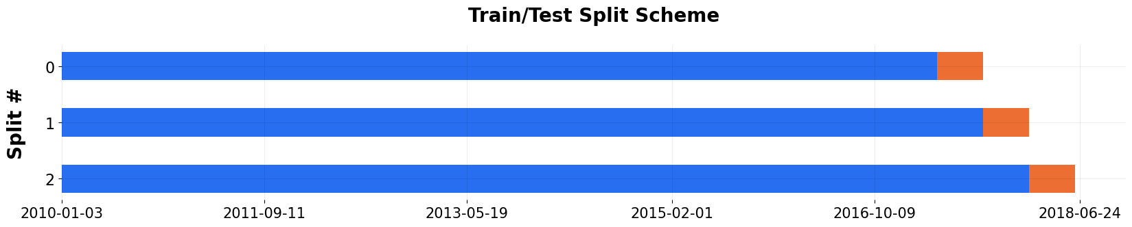
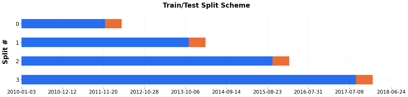
Users can visualize the splits using the internal plot() function. One may notice that the last few data points may not be included in the last split, which is expected when min_train_len is specified.

_ = ex_splitter.plot()

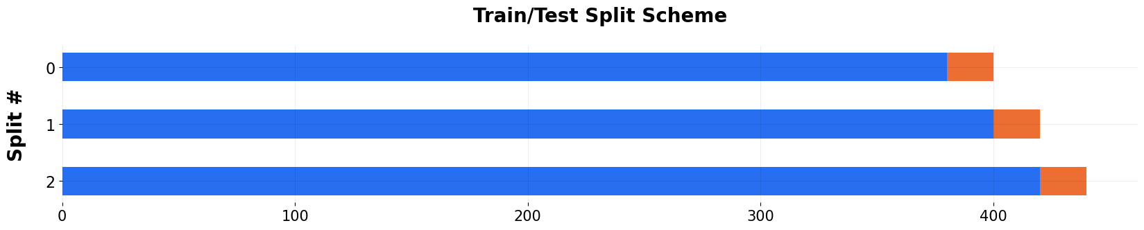
If users want to visualize the scheme in terms of indcies, one can do the following.

_ = ex_splitter.plot(show_index=True)

Rolling window

# configs
min_train_len = 380 # in case of rolling window, this specify the length of window length
forecast_len = 20 # length forecast window
incremental_len = 20 # step length for moving forward

roll_splitter = TimeSeriesSplitter(data,
                                   min_train_len=min_train_len,
                                   incremental_len=incremental_len,
                                   forecast_len=forecast_len,
                                   window_type='rolling', date_col='week')

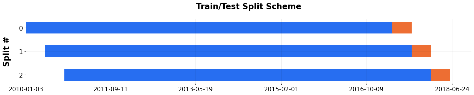
Users can visualize the splits, green is training window and yellow it the forecasting window. The window length is always 380, while the starting point moves forward 20 weeks each steps.

_ = roll_splitter.plot()

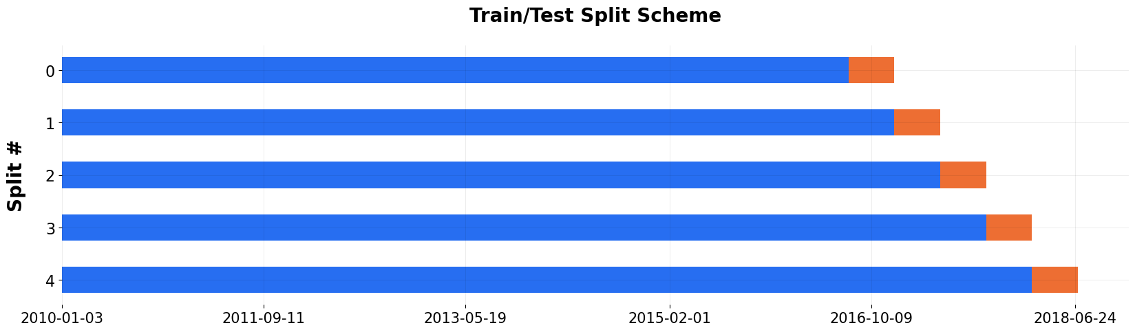
Specifying number of splits

User can also define number of splits using n_splits instead of specifying minimum training length. That way, minimum training length will be automatically calculated.

ex_splitter2 = TimeSeriesSplitter(data,
                                  min_train_len=min_train_len,
                                  incremental_len=incremental_len,
                                  forecast_len=forecast_len,
                                  n_splits=5,
                                  window_type='expanding', date_col='week')

_ = ex_splitter2.plot()

TimeSeriesSplitter as generator

TimeSeriesSplitter is implemented as a generator, therefore users can call split() to loop through it. It comes handy even for tasks other than backtest.

 for train_df, test_df, scheme, key in roll_splitter.split():
        print('Initial Claim slice {} rolling mean:{:.3f}'.format(key, train_df['claims'].mean()))

Initial Claim slice 0 rolling mean:12.712
Initial Claim slice 1 rolling mean:12.671
Initial Claim slice 2 rolling mean:12.647

Create a BackTester

To actually run backtest, first let’s initialize a DLT model and a BackTester. You pass in TimeSeriesSplitter parameters to BackTester.

# instantiate a model
dlt = DLT(
    date_col='week',
    response_col='claims',
    regressor_col=['trend.unemploy', 'trend.filling', 'trend.job'],
    seasonality=52,
    estimator='stan-map',
    # reduce number of messages
    verbose=False,
)

# configs
min_train_len = 100
forecast_len = 20
incremental_len = 100
window_type = 'expanding'

bt = BackTester(
    model=dlt,
    df=data,
    min_train_len=min_train_len,
    incremental_len=incremental_len,
    forecast_len=forecast_len,
    window_type=window_type,
)

Backtest fit and predict

The most expensive portion of backtesting is fitting the model iteratively. Thus, users can separate the API calls for fit_predict and score to avoid redundant computation for multiple metrics or scoring methods

bt.fit_predict()

Once fit_predict() is called, the fitted models and predictions can be easily retrieved from BackTester. Here the data is grouped by the date, split_key, and whether or not that observation is part of the training or test data

predicted_df = bt.get_predicted_df()
predicted_df.head()

	date	actual	prediction	training_data	split_key
0	2010-01-03	13.386595	13.386595	True	0
1	2010-01-10	13.624218	13.649157	True	0
2	2010-01-17	13.398741	13.373225	True	0
3	2010-01-24	13.137549	13.210564	True	0
4	2010-01-31	13.196760	13.187855	True	0

A plotting utility is also provided to visualize the predictions against the actuals for each split.

plot_bt_predictions(predicted_df, metrics=smape, ncol=2, include_vline=True);

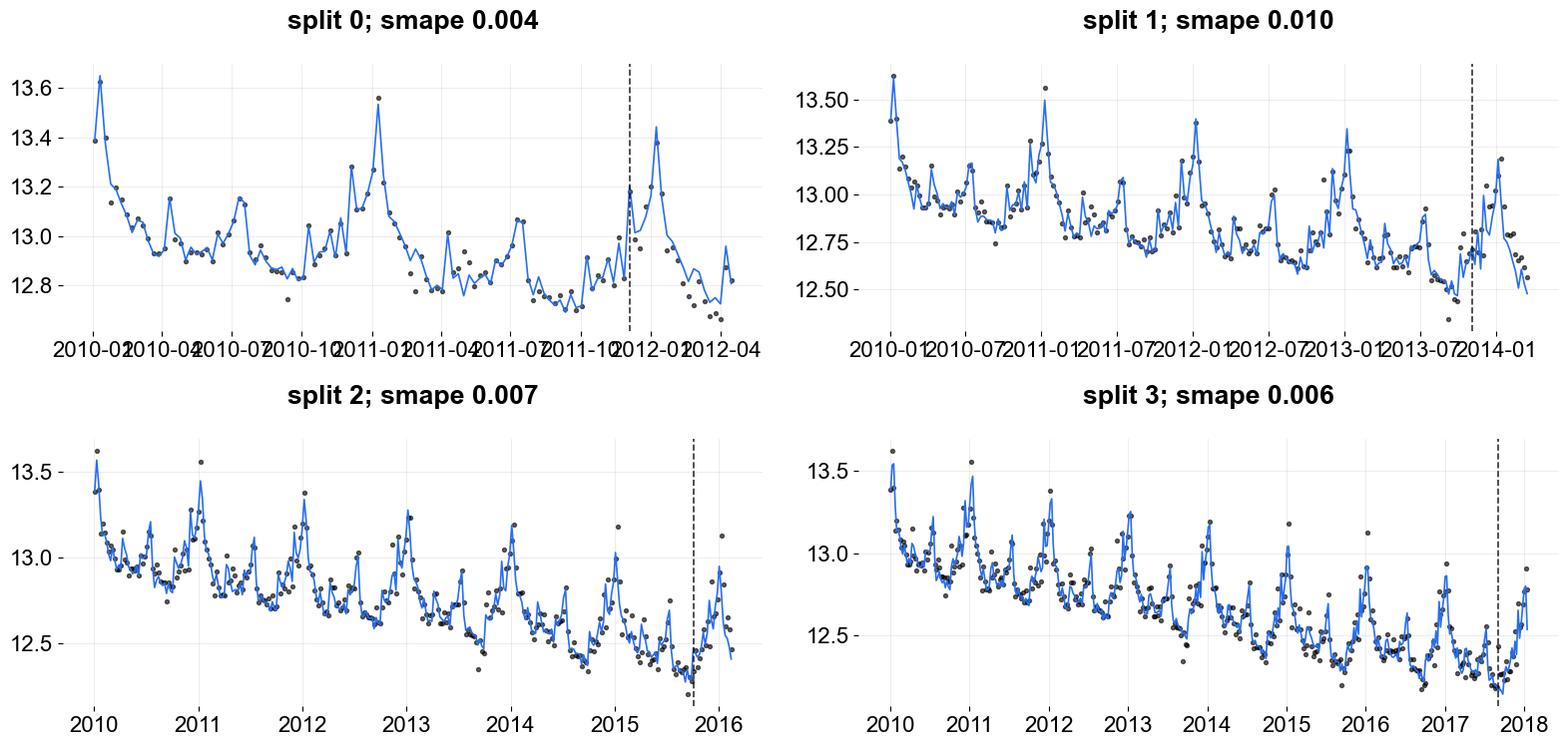
Users might find this useful for any custom computations that may need to be performed on the set of predicted data. Note that the columns are renamed to generic and consistent names.

Sometimes, it might be useful to match the data back to the original dataset for ad-hoc diagnostics. This can easily be done by merging back to the original dataset

predicted_df.merge(data, left_on='date', right_on='week')

	date	actual	prediction	training_data	split_key	week	claims	trend.unemploy	trend.filling	trend.job	sp500	vix
0	2010-01-03	13.386595	13.386595	True	0	2010-01-03	13.386595	0.219882	-0.318452	0.117500	-0.417633	0.122654
1	2010-01-03	13.386595	13.386595	True	1	2010-01-03	13.386595	0.219882	-0.318452	0.117500	-0.417633	0.122654
2	2010-01-03	13.386595	13.386595	True	2	2010-01-03	13.386595	0.219882	-0.318452	0.117500	-0.417633	0.122654
3	2010-01-03	13.386595	13.386595	True	3	2010-01-03	13.386595	0.219882	-0.318452	0.117500	-0.417633	0.122654
4	2010-01-10	13.624218	13.649157	True	0	2010-01-10	13.624218	0.219882	-0.194838	0.168794	-0.425480	0.110445
...	...	...	...	...	...	...	...	...	...	...	...	...
1075	2017-12-17	12.568616	12.566429	False	3	2017-12-17	12.568616	0.298663	0.248654	-0.216869	0.434042	-0.482380
1076	2017-12-24	12.691451	12.675786	False	3	2017-12-24	12.691451	0.328516	0.233616	-0.358839	0.430410	-0.373389
1077	2017-12-31	12.769532	12.783315	False	3	2017-12-31	12.769532	0.503457	0.069313	-0.092571	0.456087	-0.553539
1078	2018-01-07	12.908227	12.800098	False	3	2018-01-07	12.908227	0.527849	0.051295	0.029532	0.471673	-0.456456
1079	2018-01-14	12.777193	12.536719	False	3	2018-01-14	12.777193	0.465717	0.032946	0.006275	0.480271	-0.352770

1080 rows × 12 columns

Backtest Scoring

The main purpose of BackTester are the evaluation metrics. Some of the most widely used metrics are implemented and built into the BackTester API.

The default metric list is smape, wmape, mape, mse, mae, rmsse.

bt.score()

	metric_name	metric_values	is_training_metric
0	smape	0.006787	False
1	wmape	0.006785	False
2	mape	0.006770	False
3	mse	0.013098	False
4	mae	0.086193	False
5	rmsse	0.816876	False

It is possible to filter for only specific metrics of interest, or even implement your own callable and pass into the score() method. For example, see this function that uses last observed value as a predictor and computes the mse. Or naive_error which computes the error as the delta between predicted values and the training period mean.

Note these are not really useful error metrics, just showing some examples of callables you can use ;)

def mse_naive(test_actual):
    actual = test_actual[1:]
    prediction = test_actual[:-1]
    return np.mean(np.square(actual - prediction))

def naive_error(train_actual, test_prediction):
    train_mean = np.mean(train_actual)
    return np.mean(np.abs(test_prediction - train_mean))

bt.score(metrics=[mse_naive, naive_error])

	metric_name	metric_values	is_training_metric
0	mse_naive	0.019628	False
1	naive_error	0.230727	False

It doesn’t take additional time to refit and predict the model, since the results are stored when fit_predict() is called. Check docstrings for function criteria that is required for it to be supported with this api.

In some cases, users may want to evaluate our metrics on both train and test data. To do this you can call score again with the following indicator

bt.score(include_training_metrics=True)

	metric_name	metric_values	is_training_metric
0	smape	0.006787	False
1	wmape	0.006785	False
2	mape	0.006770	False
3	mse	0.013098	False
4	mae	0.086193	False
5	rmsse	0.816876	False
6	smape	0.002739	True
7	wmape	0.002742	True
8	mape	0.002738	True
9	mse	0.003116	True
10	mae	0.035042	True

Backtest Get Models

In cases where BackTester doesn’t cut it or for more custom use-cases, there’s an interface to export the TimeSeriesSplitter and predicted data, as shown earlier. It’s also possible to get each of the fitted models for deeper diving

fitted_models = bt.get_fitted_models()

model_1 = fitted_models[0]
model_1.get_regression_coefs()

	regressor	regressor_sign	coefficient
0	trend.unemploy	Regular	-0.048311
1	trend.filling	Regular	-0.120104
2	trend.job	Regular	0.028545

BackTester composes a TimeSeriesSplitter within it, but TimeSeriesSplitter can also be created on its own as a standalone object. See section below on TimeSeriesSplitter for more details on how to use the splitter.

All of the additional TimeSeriesSplitter args can also be passed into BackTester on instantiation

ts_splitter = bt.get_splitter()
_ = ts_splitter.plot()

Hyperparameter Tunning

After seeing the results from the backtest, users may wish to fine tune the hyperparameters. Orbit also provide a grid_search_orbit utilities for parameter searching. It uses Backtester under the hood so users can compare backtest metrics for different parameters combination.

To have a consistent outlook here, users need to make sure an updated version of ipywidgets is installed.

from orbit.utils.params_tuning import grid_search_orbit

# defining the search space for level smoothing paramter and seasonality smooth paramter
param_grid = {
    'level_sm_input': [0.3, 0.5, 0.8],
    'seasonality_sm_input': [0.3, 0.5, 0.8],
}

# configs
min_train_len = 380 # in case of rolling window, this specify the length of window length
forecast_len = 20 # length forecast window
incremental_len = 20 # step length for moving forward
best_params, tuned_df = grid_search_orbit(
    param_grid,
    model=dlt,
    df=data,
    min_train_len=min_train_len,
    incremental_len=incremental_len,
    forecast_len=forecast_len,
    metrics=None,
    criteria="min",
    verbose=False,
)

tuned_df.head() # backtest output for each parameter searched

	level_sm_input	seasonality_sm_input	metrics
0	0.3	0.3	0.004909
1	0.3	0.5	0.004058
2	0.3	0.8	0.003609
3	0.5	0.3	0.007908
4	0.5	0.5	0.006306

best_params # output best parameters

[{'level_sm_input': 0.3, 'seasonality_sm_input': 0.8}]