EDA Utilities¶

In this section, we will introduce a rich set of plotting functions in orbit for the EDA (exploratory data analysis) purpose. The plots include

Time series heatmap
Correlation heatmap
Dual axis time series plot
Wrap plot

[1]:

import seaborn as sns
from matplotlib import pyplot as plt
import pandas as pd
import numpy as np

import orbit
from orbit.utils.dataset import load_iclaims
from orbit.eda import eda_plot

[2]:

print(orbit.__version__)

1.1.3

[3]:

df = load_iclaims()
df['week'] = pd.to_datetime(df['week'])

[4]:

df.head()

[4]:

	week	claims	trend.unemploy	trend.filling	trend.job	sp500	vix
0	2010-01-03	13.386595	0.219882	-0.318452	0.117500	-0.417633	0.122654
1	2010-01-10	13.624218	0.219882	-0.194838	0.168794	-0.425480	0.110445
2	2010-01-17	13.398741	0.236143	-0.292477	0.117500	-0.465229	0.532339
3	2010-01-24	13.137549	0.203353	-0.194838	0.106918	-0.481751	0.428645
4	2010-01-31	13.196760	0.134360	-0.242466	0.074483	-0.488929	0.487404

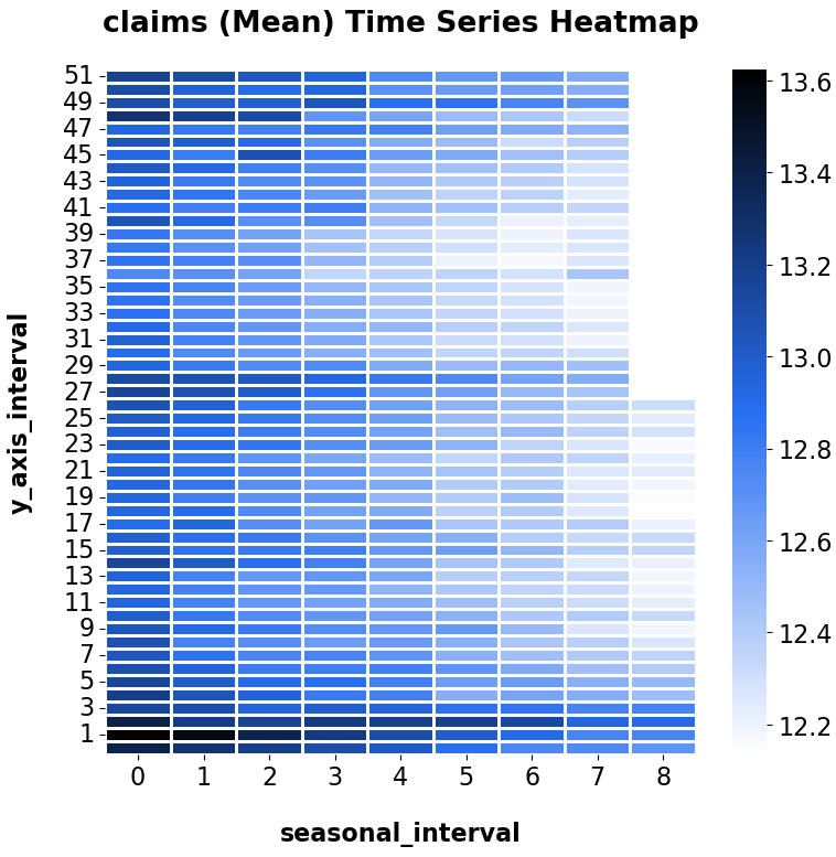
Time series heat map¶

[5]:

_ = eda_plot.ts_heatmap(df = df, date_col = 'week', seasonal_interval=52, value_col='claims')

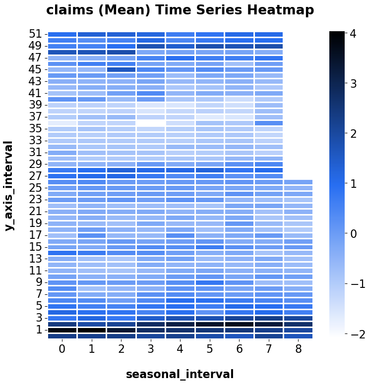
../_images/tutorials_exploratory_data_analysis_6_0.png

[6]:

_ = eda_plot.ts_heatmap(df = df, date_col = 'week',  seasonal_interval=52, value_col='claims', normalization=True)

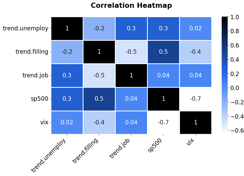
../_images/tutorials_exploratory_data_analysis_7_0.png

Correlation heatmap¶

[7]:

var_list = ['trend.unemploy', 'trend.filling', 'trend.job', 'sp500', 'vix']
_ = eda_plot.correlation_heatmap(df, var_list = var_list,
                                 fig_width=10, fig_height=6)

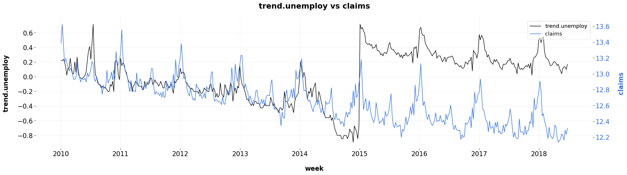
../_images/tutorials_exploratory_data_analysis_9_0.png

Dual axis time series plot¶

[8]:

_ = eda_plot.dual_axis_ts_plot(df=df, var1='trend.unemploy', var2='claims', date_col='week')

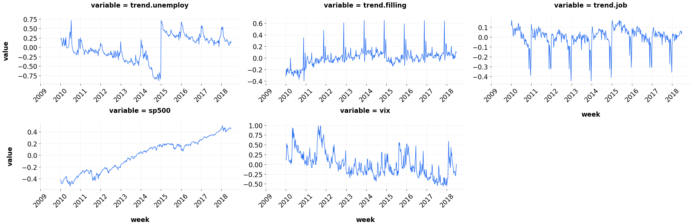
../_images/tutorials_exploratory_data_analysis_11_0.png

Wrap plots for quick glance of data patterns¶

[9]:

var_list=['week', 'trend.unemploy', 'trend.filling', 'trend.job', 'sp500', 'vix']
df[var_list].melt(id_vars = ['week'])

[9]:

	week	variable	value
0	2010-01-03	trend.unemploy	0.219882
1	2010-01-10	trend.unemploy	0.219882
2	2010-01-17	trend.unemploy	0.236143
3	2010-01-24	trend.unemploy	0.203353
4	2010-01-31	trend.unemploy	0.134360
...	...	...	...
2210	2018-05-27	vix	-0.175192
2211	2018-06-03	vix	-0.275119
2212	2018-06-10	vix	-0.291676
2213	2018-06-17	vix	-0.152422
2214	2018-06-24	vix	0.003284

2215 rows × 3 columns

[10]:

_ = eda_plot.wrap_plot_ts(df, 'week', var_list)

../_images/tutorials_exploratory_data_analysis_14_0.png