Regression Penalties in DLT
This notebook continues to discuss regression problems with DLT and covers various penalties:
fixed-ridgeauto-ridgelasso
Generally speaking, regression coefficients are more robust under full Bayesian sampling and estimation. The default setting estimator='stan-mcmc' will be used in this tutorial. Besides, a fixed and small smoothing parameters are used such as level_sm_input=0.01 and slope_sm_input=0.01 to facilitate high dimensional regression.
[1]:
%matplotlib inline

import matplotlib.pyplot as plt
import numpy as np

import orbit
from orbit.utils.dataset import load_iclaims
from orbit.models import DLT
from orbit.diagnostics.plot import plot_predicted_data
from orbit.constants.palette import OrbitPalette
[2]:
print(orbit.__version__)
1.1.3
Regression on Simulated Dataset
A simulated dataset is used to demonstrate sparse regression.
[3]:
import pandas as pd
from orbit.utils.simulation import make_trend, make_regression
from orbit.diagnostics.metrics import mse
A few utilities from the package is used to generate simulated data. For details, please refer to the API doc. In brief, the process generates observations \(y\) such that
\[y_t = l_t + \sum_p^{P} \beta_p x_{t, p}\]
\[\text{ for } t = 1,2, \cdots , T\]
where
Regular Regression
To begin with, the setting \(P=10\) and \(T=100\) is used.
[4]:
NUM_OF_REGRESSORS = 10
SERIES_LEN = 50
SEED = 20210101
# sample some coefficients
COEFS = np.random.default_rng(SEED).uniform(-1, 1, NUM_OF_REGRESSORS)
trend = make_trend(SERIES_LEN, rw_loc=0.01, rw_scale=0.1)
x, regression, coefs = make_regression(series_len=SERIES_LEN, coefs=COEFS)
print(regression.shape, x.shape)
(50,) (50, 10)
[5]:
# combine trend and the regression
y = trend + regression
[6]:
x_cols = [f"x{x}" for x in range(1, NUM_OF_REGRESSORS + 1)]
response_col = "y"
dt_col = "date"
obs_matrix = np.concatenate([y.reshape(-1, 1), x], axis=1)
# make a data frame for orbit inputs
df = pd.DataFrame(obs_matrix, columns=[response_col] + x_cols)
# make some dummy date stamp
dt = pd.date_range(start='2016-01-04', periods=SERIES_LEN, freq="1W")
df['date'] = dt
df.shape
[6]:
(50, 12)
Here is a peek on the coefficients.
[7]:
coefs
[7]:
array([ 0.38372743, -0.21084054,  0.5404565 , -0.21864409,  0.85529298,
       -0.83838077, -0.54550632,  0.80367924, -0.74643654, -0.26626975])
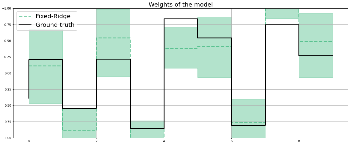
By default, regression_penalty is set as fixed-ridge i.e.
with a default \(\mu_j = 0\) and \(\sigma_j = 1\)
Fixed Ridge Penalty
[8]:
%%time
dlt_fridge = DLT(
    response_col=response_col,
    date_col=dt_col,
    regressor_col=x_cols,
    seed=SEED,
    # this is default
    regression_penalty='fixed_ridge',
    # fixing the smoothing parameters to learn regression coefficients more effectively
    level_sm_input=0.01,
    slope_sm_input=0.01,
    num_warmup=4000,
)
dlt_fridge.fit(df=df)
INFO:orbit:Sampling (PyStan) with chains: 4, cores: 8, temperature: 1.000, warmups (per chain): 1000 and samples(per chain): 25.
WARNING:pystan:n_eff / iter below 0.001 indicates that the effective sample size has likely been overestimated
WARNING:pystan:Rhat above 1.1 or below 0.9 indicates that the chains very likely have not mixed
CPU times: user 46.3 ms, sys: 43 ms, total: 89.3 ms
Wall time: 1.4 s
[8]:
<orbit.forecaster.full_bayes.FullBayesianForecaster at 0x177f1f610>
[9]:
coef_fridge = np.quantile(dlt_fridge._posterior_samples['beta'], q=[0.05, 0.5, 0.95], axis=0 )
lw=3
idx = np.arange(NUM_OF_REGRESSORS)
plt.figure(figsize=(20, 8))
plt.title("Weights of the model", fontsize=20)
plt.plot(idx, coef_fridge[1], color=OrbitPalette.GREEN.value, linewidth=lw,  drawstyle='steps', label='Fixed-Ridge', alpha=0.5, linestyle='--')
plt.fill_between(idx, coef_fridge[0], coef_fridge[2], step='pre', alpha=0.3, color=OrbitPalette.GREEN.value)
plt.plot(coefs, color="black", linewidth=lw,  drawstyle='steps', label="Ground truth")
plt.ylim(1, -1)
plt.legend(prop={'size': 20})
plt.grid()
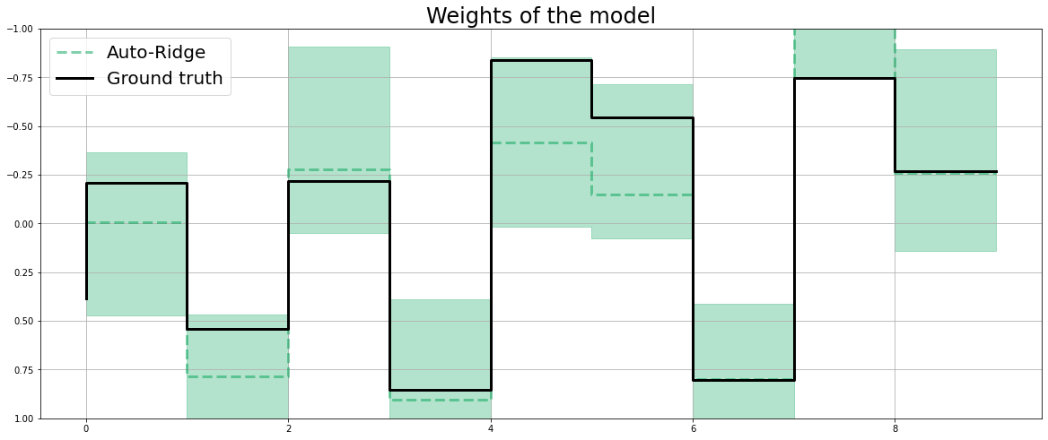
Auto-Ridge Penalty
Users can also set the regression_penalty to be auto-ridge in case users are not sure what to set for the regressor_sigma_prior.
Instead of using fixed scale in the coefficients prior, a prior can be assigned to them, i.e.
This can be done by setting regression_penalty="auto_ridge" with the argument auto_ridge_scale (default of 0.5) set the prior \(\alpha\). A higher adapt_delta is recommend to reduce divergence. Check here for details of adapt_delta.
[10]:
%%time
dlt_auto_ridge = DLT(
    response_col=response_col,
    date_col=dt_col,
    regressor_col=x_cols,
    seed=SEED,
    # this is default
    regression_penalty='auto_ridge',
    # fixing the smoothing parameters to learn regression coefficients more effectively
    level_sm_input=0.01,
    slope_sm_input=0.01,
    num_warmup=4000,
    # reduce divergence
    stan_mcmc_control={'adapt_delta':0.9},
)
dlt_auto_ridge.fit(df=df)
INFO:orbit:Sampling (PyStan) with chains: 4, cores: 8, temperature: 1.000, warmups (per chain): 1000 and samples(per chain): 25.
WARNING:pystan:n_eff / iter below 0.001 indicates that the effective sample size has likely been overestimated
WARNING:pystan:Rhat above 1.1 or below 0.9 indicates that the chains very likely have not mixed
CPU times: user 210 ms, sys: 84.7 ms, total: 295 ms
Wall time: 2.53 s
[10]:
<orbit.forecaster.full_bayes.FullBayesianForecaster at 0x178041f70>
[11]:
coef_auto_ridge = np.quantile(dlt_auto_ridge._posterior_samples['beta'], q=[0.05, 0.5, 0.95], axis=0 )
lw=3
idx = np.arange(NUM_OF_REGRESSORS)
plt.figure(figsize=(20, 8))
plt.title("Weights of the model", fontsize=24)
plt.plot(idx, coef_auto_ridge[1], color=OrbitPalette.GREEN.value, linewidth=lw,  drawstyle='steps', label='Auto-Ridge', alpha=0.5, linestyle='--')
plt.fill_between(idx, coef_auto_ridge[0], coef_auto_ridge[2], step='pre', alpha=0.3, color=OrbitPalette.GREEN.value)
plt.plot(coefs, color="black", linewidth=lw,  drawstyle='steps', label="Ground truth")
plt.ylim(1, -1)
plt.legend(prop={'size': 20})
plt.grid();
[12]:
print('Fixed Ridge MSE:{:.3f}\nAuto Ridge MSE:{:.3f}'.format(
    mse(coef_fridge[1], coefs), mse(coef_auto_ridge[1], coefs)
))
Fixed Ridge MSE:0.103
Auto Ridge MSE:0.075
Sparse Regrssion
In reality, users usually faces a more challenging problem with a much higher \(P\) to \(N\) ratio with a sparsity specified by the parameter relevance=0.5 under the simulation process.
[13]:
NUM_OF_REGRESSORS = 50
SERIES_LEN = 50
SEED = 20210101
COEFS = np.random.default_rng(SEED).uniform(0.3, 0.5, NUM_OF_REGRESSORS)
SIGNS = np.random.default_rng(SEED).choice([1, -1], NUM_OF_REGRESSORS)
# to mimic a either zero or relative observable coefficients
COEFS = COEFS * SIGNS
trend = make_trend(SERIES_LEN, rw_loc=0.01, rw_scale=0.1)
x, regression, coefs = make_regression(series_len=SERIES_LEN, coefs=COEFS, relevance=0.5)
print(regression.shape, x.shape)
(50,) (50, 50)
[14]:
# generated sparsed coefficients
coefs
[14]:
array([ 0.        ,  0.        , -0.45404565,  0.37813559,  0.        ,
        0.        ,  0.        ,  0.48036792, -0.32535635, -0.37337302,
       -0.42474576,  0.        , -0.37000755,  0.44887456,  0.47082836,
        0.        ,  0.32678039,  0.37436121,  0.38932392,  0.40216056,
        0.        ,  0.        , -0.3076828 , -0.35036047,  0.        ,
        0.        ,  0.        ,  0.        ,  0.        ,  0.        ,
       -0.45838674,  0.3171478 ,  0.        ,  0.        ,  0.        ,
        0.        ,  0.        ,  0.41599814,  0.        , -0.30964341,
       -0.42072894,  0.36255583,  0.        , -0.39326337,  0.44455655,
        0.        ,  0.        ,  0.30064161, -0.46083203,  0.        ])
[15]:
# combine trend and the regression
y = trend + regression
[16]:
x_cols = [f"x{x}" for x in range(1, NUM_OF_REGRESSORS + 1)]
response_col = "y"
dt_col = "date"
obs_matrix = np.concatenate([y.reshape(-1, 1), x], axis=1)
# make a data frame for orbit inputs
df = pd.DataFrame(obs_matrix, columns=[response_col] + x_cols)
# make some dummy date stamp
dt = pd.date_range(start='2016-01-04', periods=SERIES_LEN, freq="1W")
df['date'] = dt
df.shape
[16]:
(50, 52)
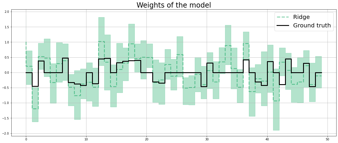
Fixed Ridge Penalty
[17]:
dlt_fridge = DLT(
    response_col=response_col,
    date_col=dt_col,
    regressor_col=x_cols,
    seed=SEED,
    level_sm_input=0.01,
    slope_sm_input=0.01,
    num_warmup=8000,
)
dlt_fridge.fit(df=df)
INFO:orbit:Sampling (PyStan) with chains: 4, cores: 8, temperature: 1.000, warmups (per chain): 2000 and samples(per chain): 25.
WARNING:pystan:n_eff / iter below 0.001 indicates that the effective sample size has likely been overestimated
WARNING:pystan:Rhat above 1.1 or below 0.9 indicates that the chains very likely have not mixed
[17]:
<orbit.forecaster.full_bayes.FullBayesianForecaster at 0x1783c0340>
[18]:
coef_fridge = np.quantile(dlt_fridge._posterior_samples['beta'], q=[0.05, 0.5, 0.95], axis=0 )
lw=3
idx = np.arange(NUM_OF_REGRESSORS)
plt.figure(figsize=(20, 8))
plt.title("Weights of the model", fontsize=24)
plt.plot(coef_fridge[1], color=OrbitPalette.GREEN.value, linewidth=lw,  drawstyle='steps', label="Ridge", alpha=0.5, linestyle='--')
plt.fill_between(idx, coef_fridge[0], coef_fridge[2], step='pre', alpha=0.3, color=OrbitPalette.GREEN.value)
plt.plot(coefs, color="black", linewidth=lw,  drawstyle='steps', label="Ground truth")
plt.legend(prop={'size': 20})
plt.grid();
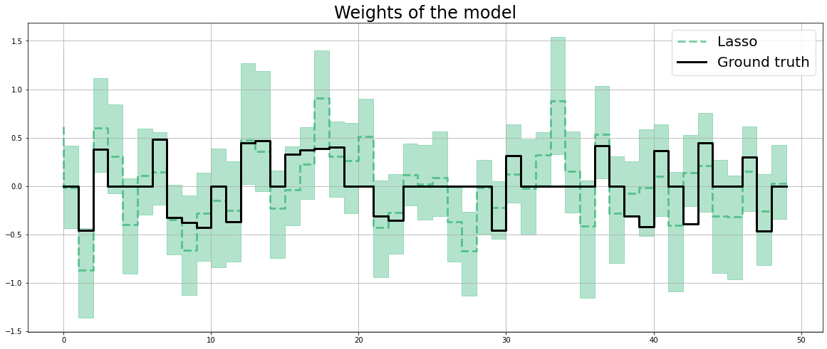
LASSO Penalty
In high \(P\) to \(N\) problems, LASS0 penalty usually shines compared to Ridge penalty.
[19]:
dlt_lasso = DLT(
    response_col=response_col,
    date_col=dt_col,
    regressor_col=x_cols,
    seed=SEED,
    regression_penalty='lasso',
    level_sm_input=0.01,
    slope_sm_input=0.01,
    num_warmup=8000,
)
dlt_lasso.fit(df=df)
INFO:orbit:Sampling (PyStan) with chains: 4, cores: 8, temperature: 1.000, warmups (per chain): 2000 and samples(per chain): 25.
WARNING:pystan:n_eff / iter below 0.001 indicates that the effective sample size has likely been overestimated
WARNING:pystan:Rhat above 1.1 or below 0.9 indicates that the chains very likely have not mixed
[19]:
<orbit.forecaster.full_bayes.FullBayesianForecaster at 0x17a5489d0>
[20]:
coef_lasso = np.quantile(dlt_lasso._posterior_samples['beta'], q=[0.05, 0.5, 0.95], axis=0 )
lw=3
idx = np.arange(NUM_OF_REGRESSORS)
plt.figure(figsize=(20, 8))
plt.title("Weights of the model", fontsize=24)
plt.plot(coef_lasso[1], color=OrbitPalette.GREEN.value, linewidth=lw,  drawstyle='steps', label="Lasso", alpha=0.5, linestyle='--')
plt.fill_between(idx, coef_lasso[0], coef_lasso[2], step='pre', alpha=0.3, color=OrbitPalette.GREEN.value)
plt.plot(coefs, color="black", linewidth=lw,  drawstyle='steps', label="Ground truth")
plt.legend(prop={'size': 20})
plt.grid();
[21]:
print('Fixed Ridge MSE:{:.3f}\nLASSO MSE:{:.3f}'.format(
    mse(coef_fridge[1], coefs), mse(coef_lasso[1], coefs)
))
Fixed Ridge MSE:0.174
LASSO MSE:0.098
Summary
This notebook covers a few choices of penalty in regression regularization. A lasso and auto-ridge can be considered in highly sparse data.