Quick Start¶

This session covers topics:

a forecast task on iclaims dataset
a simple Bayesian ETS Model using CmdStanPy
posterior distribution extraction
tools to visualize the forecast

Load Library¶

[1]:

%matplotlib inline
import matplotlib.pyplot as plt

import orbit
from orbit.utils.dataset import load_iclaims
from orbit.models import ETS
from orbit.diagnostics.plot import plot_predicted_data

/Users/towinazure/opt/miniconda3/envs/orbit39/lib/python3.9/site-packages/tqdm/auto.py:21: TqdmWarning: IProgress not found. Please update jupyter and ipywidgets. See https://ipywidgets.readthedocs.io/en/stable/user_install.html
  from .autonotebook import tqdm as notebook_tqdm

[2]:

print(orbit.__version__)

1.1.4.2

Data¶

The iclaims data contains the weekly initial claims for US unemployment (obtained from Federal Reserve Bank of St. Louis) benefits against a few related Google trend queries (unemploy, filling and job) from Jan 2010 - June 2018. This aims to demo a similar dataset from the Bayesian Structural Time Series (BSTS) model (Scott and Varian 2014).

Note that the numbers are log-log transformed for fitting purpose and the discussion of using the regressors can be found in later chapters with the Damped Local Trend (DLT) model.

[3]:

# load data
df = load_iclaims()
date_col = 'week'
response_col = 'claims'
df.dtypes

/Users/towinazure/opt/miniconda3/envs/orbit39/lib/python3.9/site-packages/orbit/utils/dataset.py:27: UserWarning: Could not infer format, so each element will be parsed individually, falling back to `dateutil`. To ensure parsing is consistent and as-expected, please specify a format.
  df = pd.read_csv(url, parse_dates=["week"])

[3]:

week              datetime64[ns]
claims                   float64
trend.unemploy           float64
trend.filling            float64
trend.job                float64
sp500                    float64
vix                      float64
dtype: object

[4]:

df.head(5)

[4]:

	week	claims	trend.unemploy	trend.filling	trend.job	sp500	vix
0	2010-01-03	13.386595	0.219882	-0.318452	0.117500	-0.417633	0.122654
1	2010-01-10	13.624218	0.219882	-0.194838	0.168794	-0.425480	0.110445
2	2010-01-17	13.398741	0.236143	-0.292477	0.117500	-0.465229	0.532339
3	2010-01-24	13.137549	0.203353	-0.194838	0.106918	-0.481751	0.428645
4	2010-01-31	13.196760	0.134360	-0.242466	0.074483	-0.488929	0.487404

Train-test split.

[5]:

test_size = 52
train_df = df[:-test_size]
test_df = df[-test_size:]

Forecasting Using Orbit¶

Orbit aims to provide an intuitive initialize-fit-predict interface for working with forecasting tasks. Under the hood, it utilizes probabilistic modeling API such as PyStan and Pyro. We first illustrate a Bayesian implementation of Rob Hyndman’s ETS (which stands for Error, Trend, and Seasonality) Model (Hyndman et. al, 2008) using PyStan.

[18]:

ets = ETS(
    response_col=response_col,
    date_col=date_col,
    seasonality=52,
    seed=2024,
    estimator="stan-mcmc",
    stan_mcmc_args={'show_progress': False},
)

[19]:

%%time
ets.fit(df=train_df)

2023-12-25 15:16:06 - orbit - INFO - Sampling (CmdStanPy) with chains: 4, cores: 8, temperature: 1.000, warmups (per chain): 225 and samples(per chain): 25.

CPU times: user 56.7 ms, sys: 23.4 ms, total: 80 ms
Wall time: 585 ms

[19]:

<orbit.forecaster.full_bayes.FullBayesianForecaster at 0x15f1d4850>

[20]:

predicted_df = ets.predict(df=test_df)

[21]:

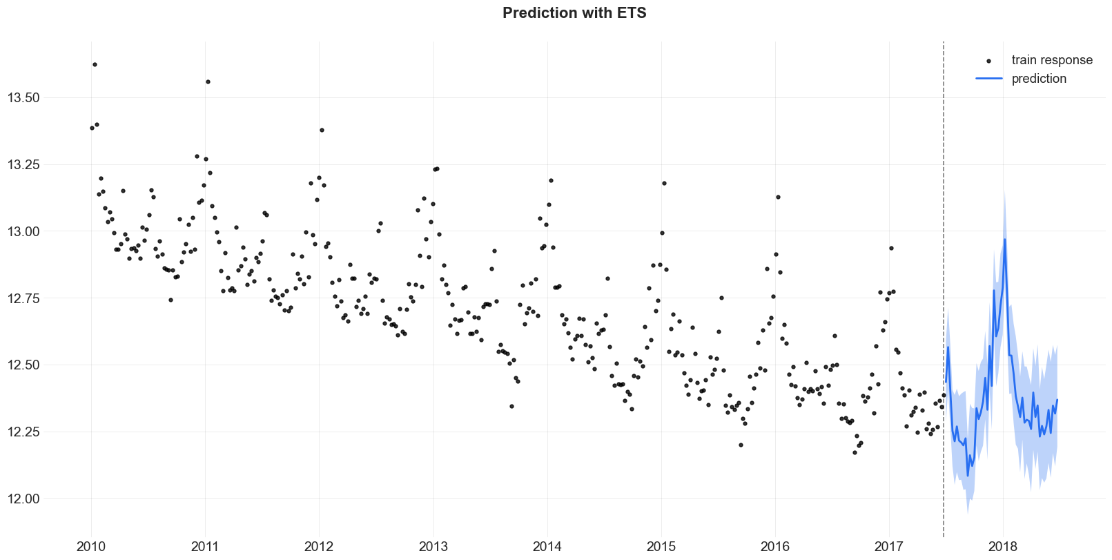
_ = plot_predicted_data(train_df, predicted_df, date_col, response_col, title='Prediction with ETS')

../_images/tutorials_quick_start_16_0.png

Extract and Analyze Posterior Samples¶

Users can use .get_posterior_samples() to extract posterior samples in an OrderedDict format.

[10]:

posterior_samples = ets.get_posterior_samples()
posterior_samples.keys()

[10]:

dict_keys(['l', 'lev_sm', 'obs_sigma', 's', 'sea_sm', 'loglk'])

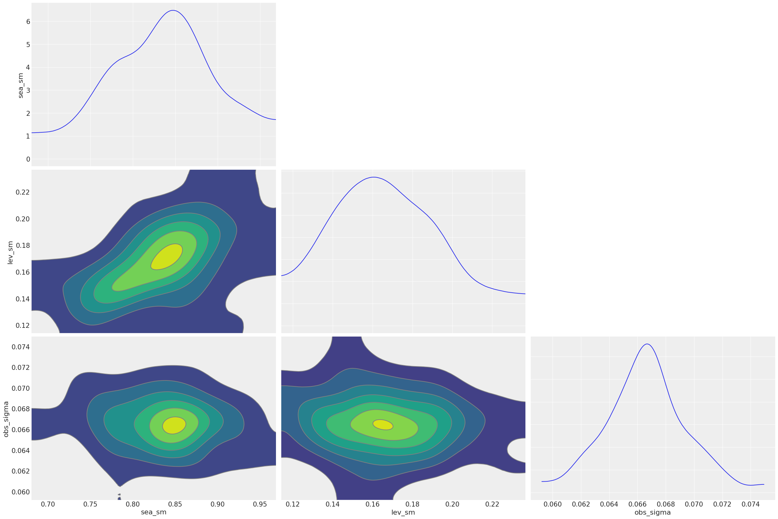
The extracted parameters posteriors are pretty much compatible diagnostic with arviz. To do that, users can set permute=False to preserve chain information.

[11]:

import arviz as az

posterior_samples = ets.get_posterior_samples(permute=False)

# example from https://arviz-devs.github.io/arviz/index.html
az.style.use("arviz-darkgrid")
az.plot_pair(
    posterior_samples,
    var_names=["sea_sm", "lev_sm", "obs_sigma"],
    kind="kde",
    marginals=True,
    textsize=15,
)
plt.show()

/Users/towinazure/opt/miniconda3/envs/orbit39/lib/python3.9/site-packages/xarray/core/utils.py:494: FutureWarning: The return type of `Dataset.dims` will be changed to return a set of dimension names in future, in order to be more consistent with `DataArray.dims`. To access a mapping from dimension names to lengths, please use `Dataset.sizes`.
  warnings.warn(

../_images/tutorials_quick_start_21_1.png

For more details in model diagnostics visualization, there is a subsequent section dedicated to it.