Damped Local Trend (DLT)
This section covers topics including:
DLT model structure
DLT global trend configurations
Adding regressors in DLT
Other configurations
[1]:
%matplotlib inline
import matplotlib.pyplot as plt

import orbit
from orbit.models import DLT
from orbit.diagnostics.plot import plot_predicted_data, plot_predicted_components
from orbit.utils.dataset import load_iclaims
[2]:
print(orbit.__version__)
1.1.4.6
Model Structure
DLT is one of the main exponential smoothing models we support in orbit. Performance is benchmarked with M3 monthly, M4 weekly dataset and some Uber internal dataset (Ng and Wang et al., 2020). The model is a fusion between the classical ETS (Hyndman et. al., 2008)) with some refinement leveraging ideas from Rlgt (Smyl et al., 2019). The
model has a structural forecast equations
with the update process
One important point is that using \(y_t\) as a log-transformed response usually yield better result, especially we can interpret such log-transformed model as a multiplicative form of the original model. Besides, there are two new additional components compared to the classical damped ETS model:
\(D(t)\) as the deterministic trend process
\(r\) as the regression component with \(x\) as the regressors
[3]:
# load log-transformed data
df = load_iclaims()
response_col = 'claims'
date_col = 'week'
Note
Just like LGT model, we also provide MAP and MCMC (full Bayesian) methods for DLT model (by specifying estimator='stan-map' or estimator='stan-mcmc' when instantiating a model).
MCMC is usually more robust but may take longer time to train. In this notebook, we will use the MAP method for illustration purpose.
Global Trend Configurations
There are a few choices of \(D(t)\) configured by global_trend_option:
linear(default)loglinearflatlogistic
Mathematically, they are expressed as such,
1. Linear:
\(D(t) = \delta_{\text{intercept}} + \delta_{\text{slope}} \cdot t\)
2. Log-linear:
\(D(t) = \delta_{\text{intercept}} + ln(\delta_{\text{slope}} \cdot t)\)
3. Logistic:
\(D(t) = L + \frac{U - L} {1 + e^{- \delta_{\text{slope}} \cdot t}}\)
4. Flat:
\(D(t) = \delta_{\text{intercept}}\)
where \(\delta_{\text{intercept}}\) and \(\delta_{\text{slope}}\) are fitted parameters and \(t\) is rescaled time-step between \(0\) and \(T\) (=number of time steps).
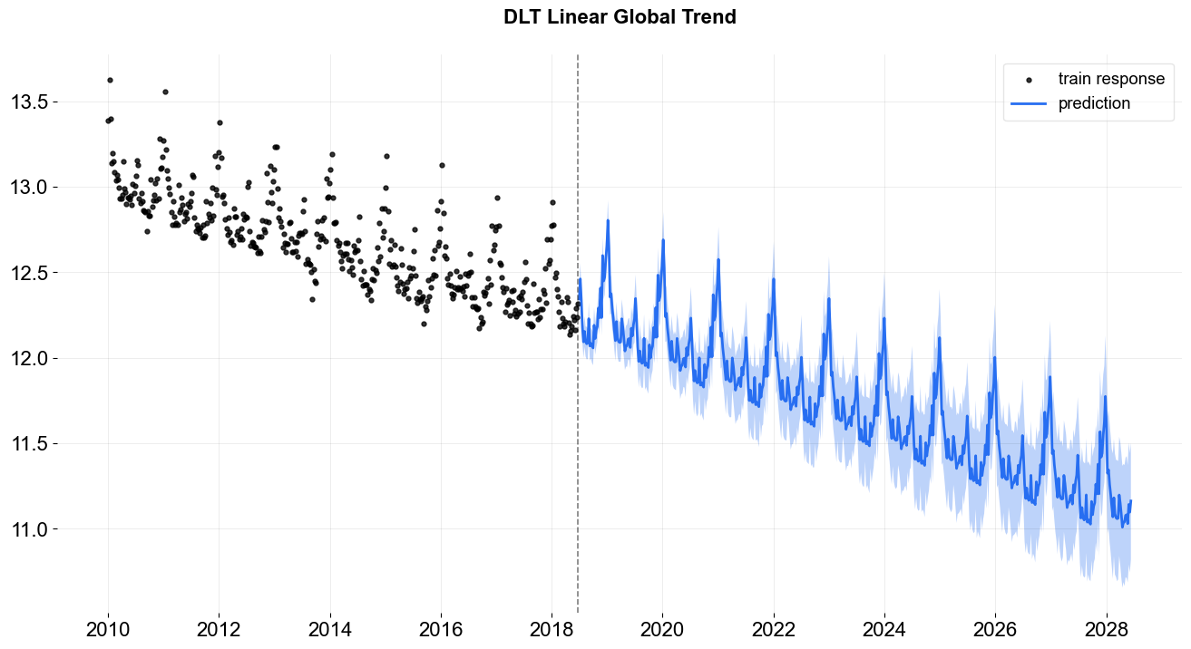
To show the difference among these options, their predictions are projected in the charts below. Note that the default is set to linear which is also used in the benchmarking process mentioned previously. During prediction, a convenient function make_future_df() is called to generate future data frame (ONLY applied when you don’t have any regressors!).
linear global trend
[4]:
%%time

dlt = DLT(
    response_col=response_col,
    date_col=date_col,
    estimator='stan-map',
    seasonality=52,
    seed=8888,
    global_trend_option='linear',
    # for prediction uncertainty
    n_bootstrap_draws=1000,
)

dlt.fit(df)
test_df = dlt.make_future_df(periods=52 * 10)
predicted_df = dlt.predict(test_df)
_ = plot_predicted_data(df, predicted_df, date_col, response_col,  title='DLT Linear Global Trend')
2024-03-19 23:38:05 - orbit - INFO - Optimizing (CmdStanPy) with algorithm: LBFGS.
CPU times: user 1.38 s, sys: 538 ms, total: 1.92 s
Wall time: 501 ms
[5]:
dlt = DLT(
    response_col=response_col,
    date_col=date_col,
    estimator='stan-mcmc',
    seasonality=52,
    seed=8888,
    global_trend_option='linear',
    # for prediction uncertainty
    n_bootstrap_draws=1000,
    stan_mcmc_args={'show_progress': False},
)

dlt.fit(df, point_method="mean")
2024-03-19 23:38:05 - orbit - INFO - Sampling (CmdStanPy) with chains: 4, cores: 8, temperature: 1.000, warmups (per chain): 225 and samples(per chain): 25.
[5]:
<orbit.forecaster.full_bayes.FullBayesianForecaster at 0x2a9230650>
One can use .get_posterior_samples() to extract the samples for all sampling parameters.
[6]:
dlt.get_posterior_samples().keys()
[6]:
dict_keys(['l', 'b', 'lev_sm', 'slp_sm', 'obs_sigma', 'nu', 'lt_sum', 's', 'sea_sm', 'gt_sum', 'gb', 'gl', 'loglk'])
[7]:
%%time
# log-linear global trend
dlt = DLT(
response_col=response_col,
date_col=date_col,
seasonality=52,
estimator='stan-map',
seed=8888,
global_trend_option='loglinear',
# for prediction uncertainty
n_bootstrap_draws=1000,
)
dlt.fit(df)
# re-use the test_df generated above
predicted_df = dlt.predict(test_df)
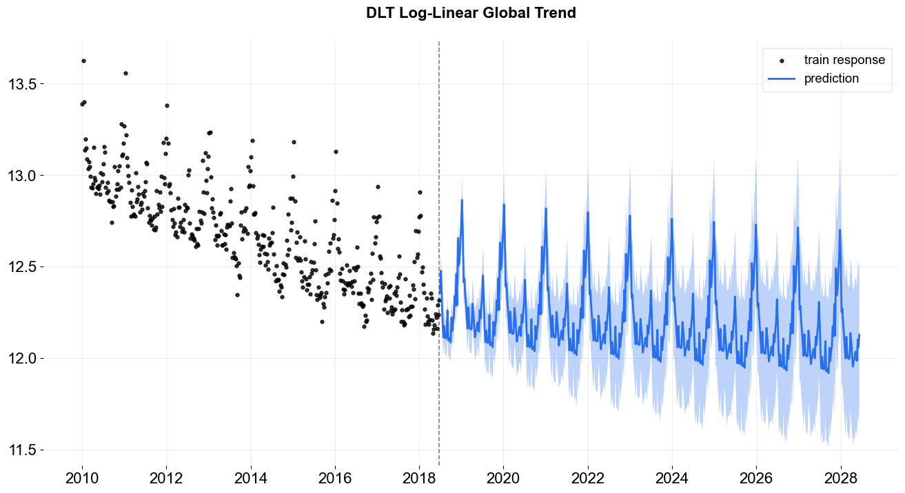
_ = plot_predicted_data(df, predicted_df, date_col, response_col, title='DLT Log-Linear Global Trend')
2024-03-19 23:38:08 - orbit - INFO - Optimizing (CmdStanPy) with algorithm: LBFGS.
CPU times: user 1.41 s, sys: 456 ms, total: 1.87 s
Wall time: 540 ms
In logistic trend, users need to specify the args global_floor and global_cap. These args are with default 0 and 1.
logistic global trend
[8]:
%%time

dlt = DLT(
    response_col=response_col,
    date_col=date_col,
    estimator='stan-map',
    seasonality=52,
    seed=8888,
    global_trend_option='logistic',
    global_cap=9999,
    global_floor=11.75,
    damped_factor=0.1,
    # for prediction uncertainty
    n_bootstrap_draws=1000,
)

dlt.fit(df)
predicted_df = dlt.predict(test_df)
ax = plot_predicted_data(df, predicted_df, date_col, response_col,
                         title='DLT Logistic Global Trend', is_visible=False);
ax.axhline(y=11.75, linestyle='--', color='orange')
ax.figure
2024-03-19 23:38:08 - orbit - INFO - Optimizing (CmdStanPy) with algorithm: LBFGS.
CPU times: user 446 ms, sys: 263 ms, total: 709 ms
Wall time: 419 ms
[8]:
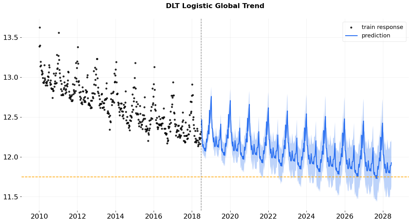
Note: Theoretically, the trend is bounded by the global_floor and global_cap. However, because of seasonality and regression, the predictions can still be slightly lower than the floor or higher than the cap.
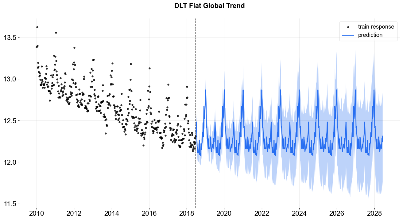
flat trend
[9]:
%%time

dlt = DLT(
    response_col=response_col,
    date_col=date_col,
    estimator='stan-map',
    seasonality=52,
    seed=8888,
    global_trend_option='flat',
    # for prediction uncertainty
    n_bootstrap_draws=1000,
)

dlt.fit(df)
predicted_df = dlt.predict(test_df)
_ = plot_predicted_data(df, predicted_df, date_col, response_col,  title='DLT Flat Global Trend')
2024-03-19 23:38:09 - orbit - INFO - Optimizing (CmdStanPy) with algorithm: LBFGS.
CPU times: user 1.33 s, sys: 264 ms, total: 1.59 s
Wall time: 681 ms
Regression
You can also add regressors into the model by specifying regressor_col. This serves the purpose of nowcasting or forecasting when exogenous regressors are known such as events and holidays. Without losing generality, the interface is set to be
where \(\mu_j = 0\) and \(\sigma_j = 1\) by default as a non-informative prior. These two parameters are set by the arguments regressor_beta_prior and regressor_sigma_prior as a list. For example,
[10]:
dlt = DLT(
response_col=response_col,
date_col=date_col,
estimator='stan-mcmc',
seed=8888,
seasonality=52,
regressor_col=['trend.unemploy', 'trend.filling'],
regressor_beta_prior=[0.1, 0.3],
regressor_sigma_prior=[0.5, 2.0],
stan_mcmc_args={'show_progress': False},
)
dlt.fit(df)
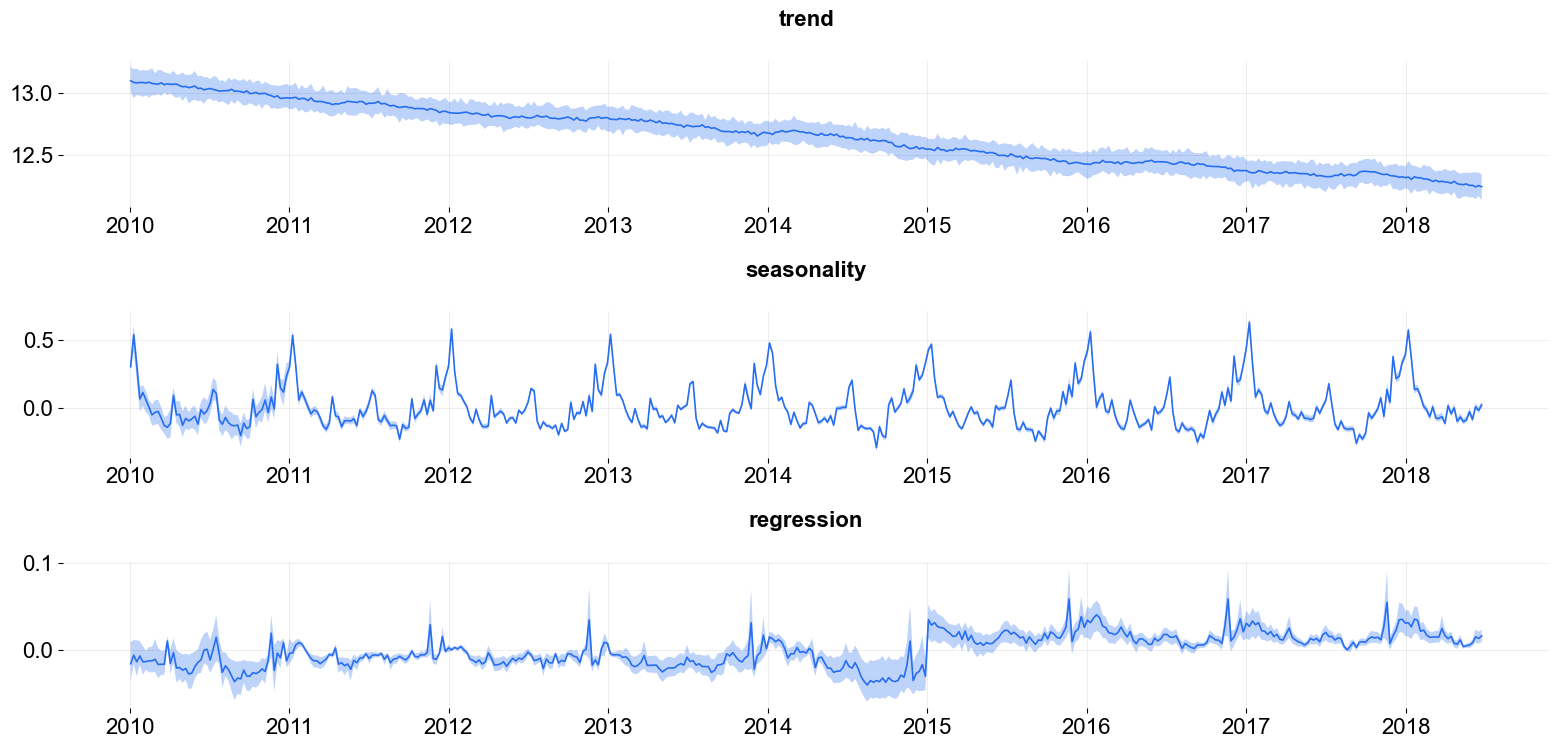
predicted_df = dlt.predict(df, decompose=True)
plot_predicted_components(predicted_df, date_col);
2024-03-19 23:38:09 - orbit - INFO - Sampling (CmdStanPy) with chains: 4, cores: 8, temperature: 1.000, warmups (per chain): 225 and samples(per chain): 25.
One can also use .get_regression_coefs to extract the regression coefficients along with the confidence interval when posterior samples are available. The default lower and upper limits are set to be .05 and .95.
[11]:
dlt.get_regression_coefs()
[11]:
| regressor | regressor_sign | coefficient | coefficient_lower | coefficient_upper | Pr(coef >= 0) | Pr(coef < 0) | |
|---|---|---|---|---|---|---|---|
| 0 | trend.unemploy | Regular | 0.052448 | 0.020843 | 0.076498 | 1.00 | 0.00 |
| 1 | trend.filling | Regular | 0.084483 | 0.012782 | 0.139546 | 0.99 | 0.01 |
There are much more configurations on regression such as the regressors sign and penalty type. They will be discussed in subsequent sections.
High Dimensional and Fourier Series Regression
In case of high dimensional regression, users can consider fixing the smoothness with a relatively small levels smoothing values e.g. setting level_sm_input=0.01. This is particularly useful in modeling higher frequency time-series such as daily and hourly data using regression on Fourier series. Check out the examples/ folder for the details.