Kernel-based Time-varying Regression - Part III¶

The tutorials I and II described the KTR model, its fitting procedure, visualizations and diagnostics / validation methods . This tutorial covers more KTR configurations for advanced users. In particular, it describes how to use knots to model change points in the seasonality and regression coefficients.

For more detail on this see Ng, Wang and Dai (2021)., which describes how KTR knots can be thought of as change points. This highlights a similarity between KTR and Facebook’s Prophet package which introduces the change point detection on levels.

Part III covers different KTR arguments to specify knots position:

level_segements
level_knot_distance
level_knot_dates

[1]:

import pandas as pd
import numpy as np
from math import pi
import matplotlib.pyplot as plt

import orbit
from orbit.models import KTR
from orbit.diagnostics.plot import plot_predicted_data
from orbit.utils.plot import get_orbit_style
from orbit.utils.dataset import load_iclaims

%matplotlib inline
pd.set_option('display.float_format', lambda x: '%.5f' % x)

[2]:

print(orbit.__version__)

1.1.4.6

Fitting with iClaims Data¶

The iClaims data set gives the weekly log number of claims and several regressors.

[3]:

# without the endate, we would get end date='2018-06-24' to make our tutorial consistent with the older version
df = load_iclaims(end_date='2020-11-29')

DATE_COL = 'week'
RESPONSE_COL = 'claims'

print(df.shape)
df.head()

(570, 7)

[3]:

	week	claims	trend.unemploy	trend.filling	trend.job	sp500	vix
0	2010-01-03	13.38660	0.03493	-0.34414	0.12802	-0.53745	0.08456
1	2010-01-10	13.62422	0.03493	-0.22053	0.17932	-0.54529	0.07235
2	2010-01-17	13.39874	0.05119	-0.31817	0.12802	-0.58504	0.49424
3	2010-01-24	13.13755	0.01840	-0.22053	0.11744	-0.60156	0.39055
4	2010-01-31	13.19676	-0.05059	-0.26816	0.08501	-0.60874	0.44931

Specifying Levels Segments¶

The first way to specify the knot locations and number is the level_segements argument. This gives the number of between knot segments; since there is a knot on each end of each the total number of knots would be the number of segments plus one. To illustrate that, try level_segments=10 (line 5).

[4]:

response_col = 'claims'
date_col='week'

[5]:

ktr = KTR(
    response_col=response_col,
    date_col=date_col,

    level_segments=10,
    prediction_percentiles=[2.5, 97.5],
    seed=2020,
    estimator='pyro-svi'
)

[6]:

ktr.fit(df=df)
_ = ktr.plot_lev_knots()

2024-03-19 23:39:34 - orbit - INFO - Optimizing (CmdStanPy) with algorithm: LBFGS.
2024-03-19 23:39:34 - orbit - INFO - Using SVI (Pyro) with steps: 301, samples: 100, learning rate: 0.1, learning_rate_total_decay: 1.0 and particles: 100.
/Users/towinazure/opt/miniconda3/envs/orbit311/lib/python3.11/site-packages/torch/__init__.py:696: UserWarning: torch.set_default_tensor_type() is deprecated as of PyTorch 2.1, please use torch.set_default_dtype() and torch.set_default_device() as alternatives. (Triggered internally at /Users/runner/work/pytorch/pytorch/pytorch/torch/csrc/tensor/python_tensor.cpp:453.)
  _C._set_default_tensor_type(t)
2024-03-19 23:39:34 - orbit - INFO - step    0 loss = 176.47, scale = 0.083093
INFO:orbit:step    0 loss = 176.47, scale = 0.083093
2024-03-19 23:39:35 - orbit - INFO - step  100 loss = 113.08, scale = 0.046374
INFO:orbit:step  100 loss = 113.08, scale = 0.046374
2024-03-19 23:39:36 - orbit - INFO - step  200 loss = 113.14, scale = 0.046119
INFO:orbit:step  200 loss = 113.14, scale = 0.046119
2024-03-19 23:39:38 - orbit - INFO - step  300 loss = 113.21, scale = 0.046233
INFO:orbit:step  300 loss = 113.21, scale = 0.046233

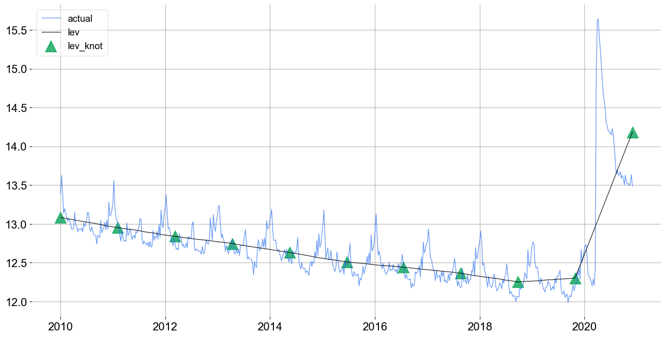
Note that there are precisely there are \(11\) knots (triangles) evenly spaced in the above chart.

Specifying Knots Distance¶

An alternative way of specifying the number of knots is the level_knot_distance argument. This argument gives the distance between knots. It can be useful as number of knots grows with the length of the time-series. Note that if the total length of the time-series is not a multiple of level_knot_distance the first segment will have a different length. For example, in a weekly data, by putting level_knot_distance=104 roughly means putting a knot once in two years.

[7]:

ktr = KTR(
    response_col=response_col,
    date_col=date_col,
    level_knot_distance=104,

    # fit a weekly seasonality
    seasonality=52,
    # high order for sharp turns on each week
    seasonality_fs_order=12,
    prediction_percentiles=[2.5, 97.5],
    seed=2020,
    estimator='pyro-svi'
)

[8]:

ktr.fit(df=df)
_ = ktr.plot_lev_knots()

2024-03-19 23:39:38 - orbit - INFO - Optimizing (CmdStanPy) with algorithm: LBFGS.
INFO:orbit:Optimizing (CmdStanPy) with algorithm: LBFGS.
2024-03-19 23:39:38 - orbit - INFO - Using SVI (Pyro) with steps: 301, samples: 100, learning rate: 0.1, learning_rate_total_decay: 1.0 and particles: 100.
INFO:orbit:Using SVI (Pyro) with steps: 301, samples: 100, learning rate: 0.1, learning_rate_total_decay: 1.0 and particles: 100.
2024-03-19 23:39:38 - orbit - INFO - step    0 loss = 145.65, scale = 0.088976
INFO:orbit:step    0 loss = 145.65, scale = 0.088976
2024-03-19 23:39:40 - orbit - INFO - step  100 loss = -5.2369, scale = 0.036939
INFO:orbit:step  100 loss = -5.2369, scale = 0.036939
2024-03-19 23:39:42 - orbit - INFO - step  200 loss = -5.3791, scale = 0.036969
INFO:orbit:step  200 loss = -5.3791, scale = 0.036969
2024-03-19 23:39:46 - orbit - INFO - step  300 loss = -5.5677, scale = 0.037689
INFO:orbit:step  300 loss = -5.5677, scale = 0.037689

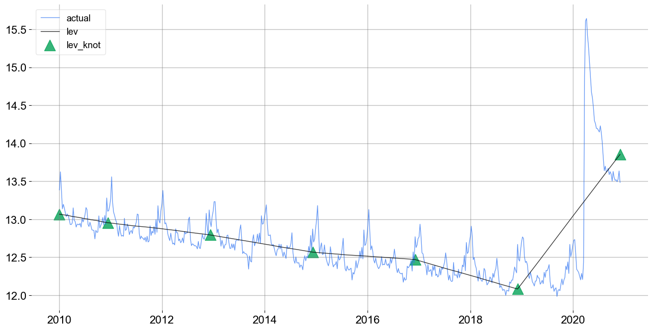
In the above chart, the knots are located about every 2-years.

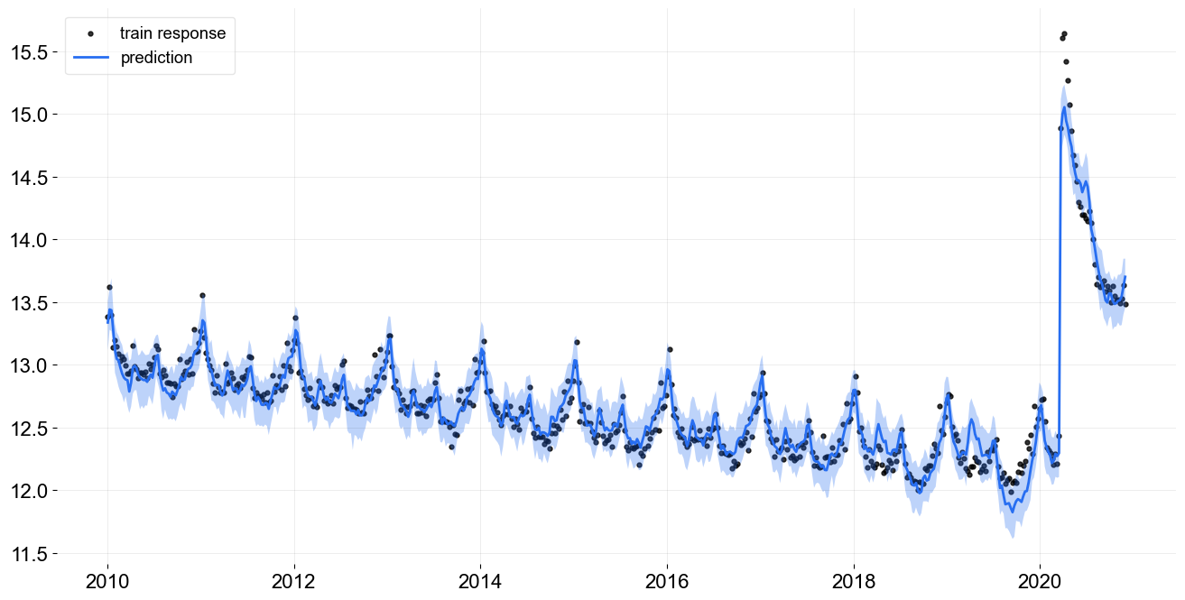
To highlight the value of the next method of configuring knot position, consider the prediction for this model show below.

[9]:

predicted_df = ktr.predict(df=df)
_ = plot_predicted_data(training_actual_df=df, predicted_df=predicted_df,  prediction_percentiles=[2.5, 97.5],
                        date_col=date_col, actual_col=response_col)

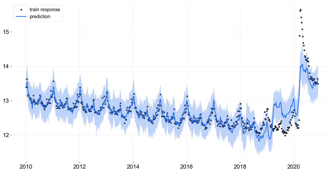
As the knots are placed evenly the model can not adequately describe the change point in early 2020. The model fit can potentially be improved by inserting knots around the sharp change points (e.g., 2020-03-15). This insertion can be done with the level_knot_dates argument described below.

Specifying Knots Dates¶

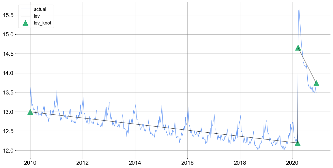
The level_knot_dates argument allows for the explicit placement of knots. It needs a string of dates; see line 4.

[10]:

ktr = KTR(
    response_col=response_col,
    date_col=date_col,
    level_knot_dates =  ['2010-01-03', '2020-03-15', '2020-03-22', '2020-11-29'],

    # fit a weekly seasonality
    seasonality=52,
    # high order for sharp turns on each week
    seasonality_fs_order=12,
    prediction_percentiles=[2.5, 97.5],
    seed=2020,
    estimator='pyro-svi'
)

[11]:

ktr.fit(df=df)

2024-03-19 23:39:46 - orbit - INFO - Optimizing (CmdStanPy) with algorithm: LBFGS.
INFO:orbit:Optimizing (CmdStanPy) with algorithm: LBFGS.
2024-03-19 23:39:46 - orbit - INFO - Using SVI (Pyro) with steps: 301, samples: 100, learning rate: 0.1, learning_rate_total_decay: 1.0 and particles: 100.
INFO:orbit:Using SVI (Pyro) with steps: 301, samples: 100, learning rate: 0.1, learning_rate_total_decay: 1.0 and particles: 100.
2024-03-19 23:39:47 - orbit - INFO - step    0 loss = 99.354, scale = 0.096314
INFO:orbit:step    0 loss = 99.354, scale = 0.096314
2024-03-19 23:39:52 - orbit - INFO - step  100 loss = -440.9, scale = 0.027049
INFO:orbit:step  100 loss = -440.9, scale = 0.027049
2024-03-19 23:39:54 - orbit - INFO - step  200 loss = -446.03, scale = 0.028019
INFO:orbit:step  200 loss = -446.03, scale = 0.028019
2024-03-19 23:39:56 - orbit - INFO - step  300 loss = -445.62, scale = 0.029141
INFO:orbit:step  300 loss = -445.62, scale = 0.029141

[11]:

<orbit.forecaster.svi.SVIForecaster at 0x2b1b1a810>

[12]:

_ = ktr.plot_lev_knots()

[13]:

predicted_df = ktr.predict(df=df)
_ = plot_predicted_data(training_actual_df=df, predicted_df=predicted_df, prediction_percentiles=[2.5, 97.5],
                        date_col=date_col, actual_col=response_col)

Note this fit is even better than the previous one using less knots. Of course, the case here is trivial because the pandemic onset is treated as known. In other cases, there may not be an obvious way to find the optimal knots dates.

Conclusion¶

This tutorial demonstrates multiple ways to customize the knots location for levels. In KTR, there are similar arguments for seasonality and regression such as seasonality_segments and regression_knot_dates and regression_segments. Due to their similarities with their knots location equivalent arguments they are not demonstrated here. However it is encouraged fro KTR users to explore them.

References¶

Ng, Wang and Dai (2021). Bayesian Time Varying Coefficient Model with Applications to Marketing Mix Modeling, arXiv preprint arXiv:2106.03322
Sean J Taylor and Benjamin Letham. 2018. Forecasting at scale. The American Statistician 72, 1 (2018), 37–45. Package version 0.7.1.