Using Pyro for Estimation
Note
Currently we are still experimenting with Pyro and support Pyro only in LGT and KTR models.
Pyro is a flexible, scalable deep probabilistic programming library built on PyTorch. Pyro was originally developed at Uber AI and is now actively maintained by community contributors, including a dedicated team at the Broad Institute.
[1]:
%matplotlib inline

import pandas as pd
import numpy as np
import matplotlib.pyplot as plt

import orbit
from orbit.models import LGT
from orbit.diagnostics.plot import plot_predicted_data
from orbit.diagnostics.plot import plot_predicted_components
from orbit.utils.dataset import load_iclaims

from orbit.constants.palette import OrbitPalette

import warnings
warnings.filterwarnings('ignore')
[2]:
print(orbit.__version__)
1.1.4.6
[3]:
df = load_iclaims()
[4]:
test_size=52
train_df=df[:-test_size]
test_df=df[-test_size:]
VI Fit and Predict
Although Pyro provides a variety of ways to optimize/sample posteriors. Currently, we only support Stochastic Variational Inference (SVI). For details, please refer to this doc.
To use SVI for LGT, specify estimator as pyro-svi.
[5]:
lgt_vi = LGT(
    response_col='claims',
    date_col='week',
    seasonality=52,
    seed=8888,
    estimator='pyro-svi',
    num_steps=101,
    num_sample=300,
    # trigger message per 50 steps
    message=50,
    learning_rate=0.1,
)
[6]:
%%time
lgt_vi.fit(df=train_df)
2024-03-19 23:40:42 - orbit - INFO - Using SVI (Pyro) with steps: 101, samples: 300, learning rate: 0.1, learning_rate_total_decay: 1.0 and particles: 100.
2024-03-19 23:40:42 - orbit - INFO - step    0 loss = 658.91, scale = 0.11635
INFO:orbit:step    0 loss = 658.91, scale = 0.11635
2024-03-19 23:40:46 - orbit - INFO - step   50 loss = -432, scale = 0.48623
INFO:orbit:step   50 loss = -432, scale = 0.48623
2024-03-19 23:40:49 - orbit - INFO - step  100 loss = -444.07, scale = 0.34976
INFO:orbit:step  100 loss = -444.07, scale = 0.34976
CPU times: user 11.8 s, sys: 33.2 s, total: 45 s
Wall time: 7.48 s
[6]:
<orbit.forecaster.svi.SVIForecaster at 0x289535f10>
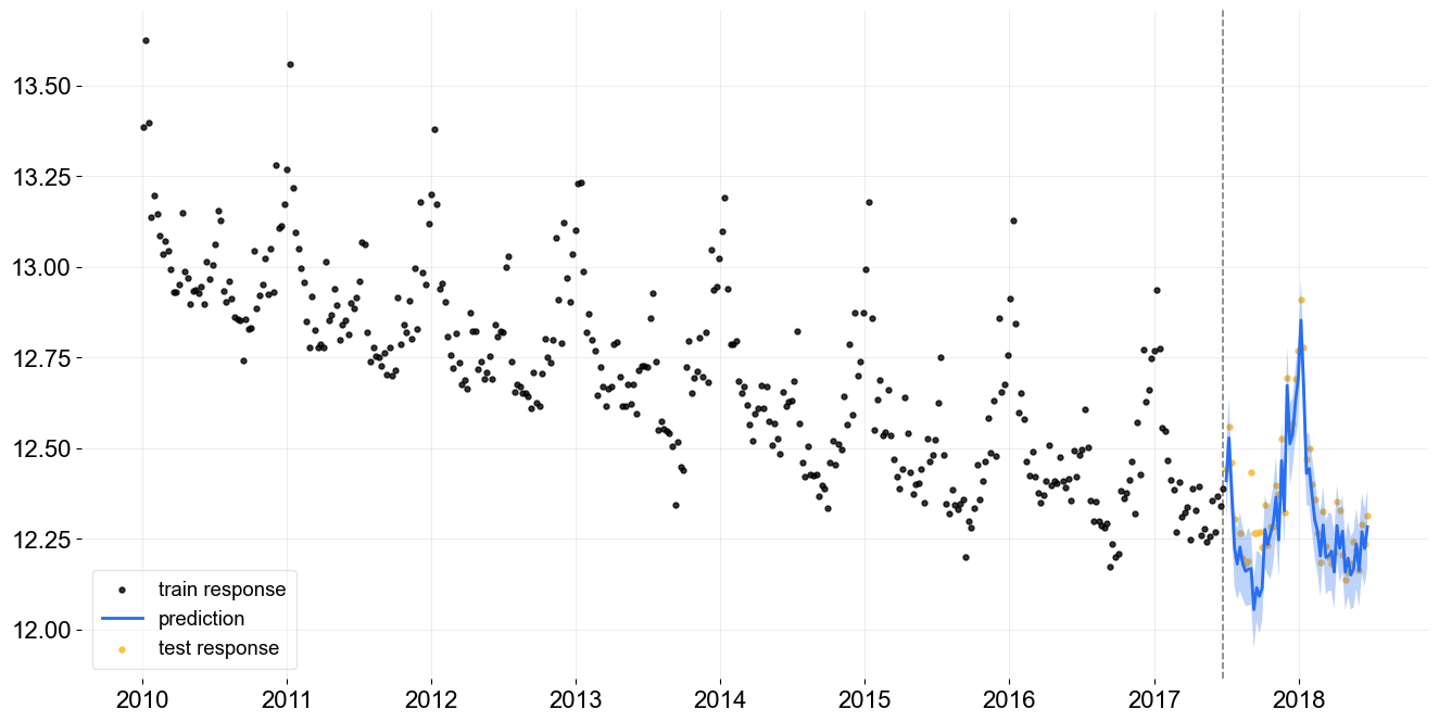
[7]:
predicted_df = lgt_vi.predict(df=test_df)
[8]:
_ = plot_predicted_data(training_actual_df=train_df, predicted_df=predicted_df,
                    date_col=lgt_vi.date_col, actual_col=lgt_vi.response_col,
                    test_actual_df=test_df)
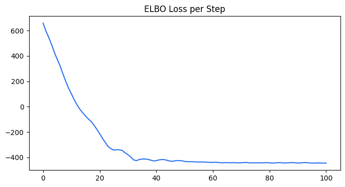
We can also extract the ELBO loss from the training metrics.
[9]:
loss_elbo = lgt_vi.get_training_metrics()['loss_elbo']
[10]:
steps = np.arange(len(loss_elbo))
plt.subplots(1, 1, figsize=(8, 4))
plt.plot(steps, loss_elbo, color=OrbitPalette.BLUE.value)
plt.title('ELBO Loss per Step')
[10]:
Text(0.5, 1.0, 'ELBO Loss per Step')