Kernel-based Time-varying Regression - Part IV
This is final tutorial on KTR. It continues from Part III with additional details on some of the advanced arguments. For other details on KTR see either the previous three tutorials or the original paper Ng, Wang and Dai (2021).
In Part IV covers advance inputs for regression including
regressors signs
time-point coefficients priors
[1]:
import pandas as pd
import numpy as np
from math import pi
import matplotlib.pyplot as plt

import orbit
from orbit.models import KTR
from orbit.diagnostics.plot import plot_predicted_components
from orbit.utils.plot import get_orbit_style
from orbit.utils.kernels import gauss_kernel
from orbit.constants.palette import OrbitPalette

%matplotlib inline
pd.set_option('display.float_format', lambda x: '%.5f' % x)
orbit_style = get_orbit_style()
plt.style.use(orbit_style);
[2]:
print(orbit.__version__)
1.1.4.6
Data
To demonstrate the effect of specifying regressors coefficients sign, it is helpful to modify the data simulation code from part II. The simulation is altered to impose strictly positive regression coefficients.
In the KTR model below, the coefficient curves are approximated with Gaussian kernels having positive values of knots. The levels are also included in the process with vector of ones as the covariates.
The parameters used to setup the data simulation are:
n: number of time stepsp: number of predictors
[3]:
np.random.seed(2021)

n = 300
p = 2
tp = np.arange(1, 301) / 300
knot_tp = np.array([1, 100, 200, 300]) / 300
beta_knot = np.array(
    [[1.0, 0.1, 0.15],
     [3.0, 0.01, 0.05],
     [3.0, 0.01, 0.05],
     [2.0, 0.05, 0.02]]
)

gk = gauss_kernel(tp, knot_tp, rho=0.2)
beta = np.matmul(gk, beta_knot)
covar_lev = np.ones((n, 1))
covar = np.concatenate((covar_lev, np.random.normal(0, 1.0, (n, p))), axis=1)\

# observation with noise
y = (covar * beta).sum(-1) + np.random.normal(0, 0.1, n)


regressor_col = ['x{}'.format(pp) for pp in range(1, p+1)]
data = pd.DataFrame(covar[:,1:], columns=regressor_col)
data['y'] = y
data['date'] = pd.date_range(start='1/1/2018', periods=len(y))
data = data[['date', 'y'] + regressor_col]
beta_col = ['beta{}'.format(pp) for pp in range(1, p+1)]
beta_data = pd.DataFrame(beta[:,1:], columns=beta_col)

data = pd.concat([data, beta_data], axis=1)
[4]:
data.tail(10)
[4]:
| date | y | x1 | x2 | beta1 | beta2 | |
|---|---|---|---|---|---|---|
| 290 | 2018-10-18 | 2.15947 | -0.62762 | 0.17840 | 0.04015 | 0.02739 |
| 291 | 2018-10-19 | 2.25871 | -0.92975 | 0.81415 | 0.04036 | 0.02723 |
| 292 | 2018-10-20 | 2.18356 | 0.82438 | -0.92705 | 0.04057 | 0.02707 |
| 293 | 2018-10-21 | 2.26948 | 1.57181 | -0.78098 | 0.04077 | 0.02692 |
| 294 | 2018-10-22 | 2.26375 | -1.07504 | -0.86523 | 0.04097 | 0.02677 |
| 295 | 2018-10-23 | 2.21349 | 0.24637 | -0.98398 | 0.04117 | 0.02663 |
| 296 | 2018-10-24 | 2.13297 | -0.58716 | 0.59911 | 0.04136 | 0.02648 |
| 297 | 2018-10-25 | 2.00949 | -2.01610 | 0.08618 | 0.04155 | 0.02634 |
| 298 | 2018-10-26 | 2.14302 | 0.33863 | -0.37912 | 0.04173 | 0.02620 |
| 299 | 2018-10-27 | 2.10795 | -0.96160 | -0.42383 | 0.04192 | 0.02606 |
Just like previous tutorials in regression, some additional args are used to describe the regressors and the scale parameters for the knots.
[5]:
ktr = KTR(
    response_col='y',
    date_col='date',
    regressor_col=regressor_col,
    regressor_init_knot_scale=[0.1] * p,
    regressor_knot_scale=[0.1] * p,
    prediction_percentiles=[2.5, 97.5],
    seed=2021,
    estimator='pyro-svi',
)
ktr.fit(df=data)
2024-03-19 23:39:37 - orbit - INFO - Optimizing (CmdStanPy) with algorithm: LBFGS.
2024-03-19 23:39:37 - orbit - INFO - Using SVI (Pyro) with steps: 301, samples: 100, learning rate: 0.1, learning_rate_total_decay: 1.0 and particles: 100.
/Users/towinazure/opt/miniconda3/envs/orbit311/lib/python3.11/site-packages/torch/__init__.py:696: UserWarning: torch.set_default_tensor_type() is deprecated as of PyTorch 2.1, please use torch.set_default_dtype() and torch.set_default_device() as alternatives. (Triggered internally at /Users/runner/work/pytorch/pytorch/pytorch/torch/csrc/tensor/python_tensor.cpp:453.)
  _C._set_default_tensor_type(t)
2024-03-19 23:39:38 - orbit - INFO - step    0 loss = -3.5592, scale = 0.085307
INFO:orbit:step    0 loss = -3.5592, scale = 0.085307
2024-03-19 23:39:39 - orbit - INFO - step  100 loss = -228.48, scale = 0.036575
INFO:orbit:step  100 loss = -228.48, scale = 0.036575
2024-03-19 23:39:40 - orbit - INFO - step  200 loss = -230.1, scale = 0.038104
INFO:orbit:step  200 loss = -230.1, scale = 0.038104
2024-03-19 23:39:41 - orbit - INFO - step  300 loss = -229.33, scale = 0.037629
INFO:orbit:step  300 loss = -229.33, scale = 0.037629
[5]:
<orbit.forecaster.svi.SVIForecaster at 0x2a836ad90>
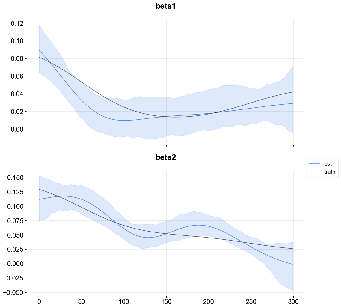
Visualization of Regression Coefficient Curves
The get_regression_coefs argument is used to extract coefficients with intervals by supplying the argument include_ci=True.
[6]:
coef_mid, coef_lower, coef_upper = ktr.get_regression_coefs(include_ci=True)
The next figure shows the overlay of the estimate on the true coefficients. Since the lower bound is below zero some of the coefficient posterior samples are negative.
[7]:
fig, axes = plt.subplots(p, 1, figsize=(12, 12), sharex=True)

x = np.arange(coef_mid.shape[0])
for idx in range(p):
    axes[idx].plot(x, coef_mid['x{}'.format(idx + 1)], label='est' if idx == 0 else "", alpha=0.8, color=OrbitPalette.BLUE.value)
    axes[idx].fill_between(x, coef_lower['x{}'.format(idx + 1)], coef_upper['x{}'.format(idx + 1)], alpha=0.15, color=OrbitPalette.BLUE.value)
    axes[idx].plot(x, data['beta{}'.format(idx + 1)], label='truth' if idx == 0 else "", alpha=0.6, color = OrbitPalette.BLACK.value)
    axes[idx].set_title('beta{}'.format(idx + 1))

fig.legend(bbox_to_anchor = (1,0.5));
Regressor Sign
Strictly positive coefficients can be imposed by using the regressor_sign arg. It can have values “=”, “-”, or “+” which denote no restriction, strictly negative, strictly positive. Note that it is possible to have a mixture by providing a list of strings one for each regressor.
[8]:
ktr = KTR(
    response_col='y',
    date_col='date',
    regressor_col=regressor_col,
    regressor_init_knot_scale=[0.1] * p,
    regressor_knot_scale=[0.1] * p,
    regressor_sign=['+'] * p,
    prediction_percentiles=[2.5, 97.5],
    seed=2021,
    estimator='pyro-svi',
)
ktr.fit(df=data)
2024-03-19 23:39:41 - orbit - INFO - Optimizing (CmdStanPy) with algorithm: LBFGS.
INFO:orbit:Optimizing (CmdStanPy) with algorithm: LBFGS.
2024-03-19 23:39:41 - orbit - INFO - Using SVI (Pyro) with steps: 301, samples: 100, learning rate: 0.1, learning_rate_total_decay: 1.0 and particles: 100.
INFO:orbit:Using SVI (Pyro) with steps: 301, samples: 100, learning rate: 0.1, learning_rate_total_decay: 1.0 and particles: 100.
2024-03-19 23:39:41 - orbit - INFO - step    0 loss = 9.7371, scale = 0.10482
INFO:orbit:step    0 loss = 9.7371, scale = 0.10482
2024-03-19 23:39:43 - orbit - INFO - step  100 loss = -231.22, scale = 0.41649
INFO:orbit:step  100 loss = -231.22, scale = 0.41649
2024-03-19 23:39:45 - orbit - INFO - step  200 loss = -230.94, scale = 0.42589
INFO:orbit:step  200 loss = -230.94, scale = 0.42589
2024-03-19 23:39:46 - orbit - INFO - step  300 loss = -230.26, scale = 0.41749
INFO:orbit:step  300 loss = -230.26, scale = 0.41749
[8]:
<orbit.forecaster.svi.SVIForecaster at 0x2b1d43810>
[9]:
coef_mid, coef_lower, coef_upper = ktr.get_regression_coefs(include_ci=True)
[10]:
fig, axes = plt.subplots(p, 1, figsize=(12, 12), sharex=True)

x = np.arange(coef_mid.shape[0])
for idx in range(p):
    axes[idx].plot(x, coef_mid['x{}'.format(idx + 1)], label='est' if idx == 0 else "", alpha=0.8, color=OrbitPalette.BLUE.value)
    axes[idx].fill_between(x, coef_lower['x{}'.format(idx + 1)], coef_upper['x{}'.format(idx + 1)], alpha=0.15, color=OrbitPalette.BLUE.value)
    axes[idx].plot(x, data['beta{}'.format(idx + 1)], label='truth' if idx == 0 else "",  alpha=0.6, color = OrbitPalette.BLACK.value)
    axes[idx].set_title('beta{}'.format(idx + 1))

fig.legend(bbox_to_anchor = (1,0.5));
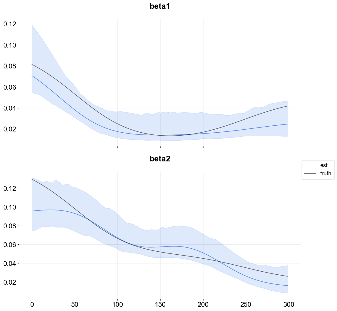
Observe the curves lie in the positive range with a slightly improved fit relative to the last model.
To conclude, it is useful to have a strictly positive range of regression coefficients if that range is known a priori. KTR allows these priors to be specified. For regression scenarios where there is no a priori knowledge of the coefficient sign it is recommended to use the default which contains both sides of the range.
Time-point coefficient priors
Users can incorporate coefficient priors for any regressor and any time period. This feature is quite useful when users have some prior knowledge or beliefs on regressor coefficients. For example, if an A/B test is conducted for a certain regressor over a specific time range, then users can ingest the priors derived from such A/B test.
This can be done by supplying a list of dictionaries via coef_prior_list. Each dict in the list should have keys as name, prior_start_tp_idx (inclusive), prior_end_tp_idx (not inclusive), prior_mean, prior_sd, and prior_regressor_col.
Below is an illustrative example by using the simulated data above.
[11]:
from copy import deepcopy
[12]:
prior_duration = 50
coef_list_dict = []
prior_idx=[
    np.arange(150, 150 + prior_duration),
    np.arange(200, 200 + prior_duration),
]
regressor_idx = range(1, p + 1)
plot_dict = {}
for i in regressor_idx:
    plot_dict[i] = {'idx': [], 'val': []}
[13]:
for idx, idx2, regressor in zip(prior_idx, regressor_idx, regressor_col):
    prior_dict = {}
    prior_dict['name'] = f'prior_{regressor}'
    prior_dict['prior_start_tp_idx'] = idx[0]
    prior_dict['prior_end_tp_idx'] = idx[-1] + 1
    prior_dict['prior_mean'] = beta[idx, idx2]
    prior_dict['prior_sd'] = [0.1] * len(idx)
    prior_dict['prior_regressor_col'] = [regressor] * len(idx)

    plot_dict[idx2]['idx'].extend(idx)
    plot_dict[idx2]['val'].extend(beta[idx, idx2])

    coef_list_dict.append(deepcopy(prior_dict))
[14]:
ktr = KTR(
    response_col='y',
    date_col='date',
    regressor_col=regressor_col,
    regressor_init_knot_scale=[0.1] * p,
    regressor_knot_scale=[0.1] * p,
    regressor_sign=['+'] * p,
    coef_prior_list = coef_list_dict,
    prediction_percentiles=[2.5, 97.5],
    seed=2021,
    estimator='pyro-svi',
)
ktr.fit(df=data)
2024-03-19 23:39:47 - orbit - INFO - Optimizing (CmdStanPy) with algorithm: LBFGS.
INFO:orbit:Optimizing (CmdStanPy) with algorithm: LBFGS.
2024-03-19 23:39:47 - orbit - INFO - Using SVI (Pyro) with steps: 301, samples: 100, learning rate: 0.1, learning_rate_total_decay: 1.0 and particles: 100.
INFO:orbit:Using SVI (Pyro) with steps: 301, samples: 100, learning rate: 0.1, learning_rate_total_decay: 1.0 and particles: 100.
2024-03-19 23:39:47 - orbit - INFO - step    0 loss = -5741.9, scale = 0.094521
INFO:orbit:step    0 loss = -5741.9, scale = 0.094521
2024-03-19 23:39:52 - orbit - INFO - step  100 loss = -7140.3, scale = 0.31416
INFO:orbit:step  100 loss = -7140.3, scale = 0.31416
2024-03-19 23:39:55 - orbit - INFO - step  200 loss = -7139.1, scale = 0.31712
INFO:orbit:step  200 loss = -7139.1, scale = 0.31712
2024-03-19 23:39:57 - orbit - INFO - step  300 loss = -7139.5, scale = 0.33039
INFO:orbit:step  300 loss = -7139.5, scale = 0.33039
[14]:
<orbit.forecaster.svi.SVIForecaster at 0x2b1eb5f10>
[15]:
coef_mid, coef_lower, coef_upper = ktr.get_regression_coefs(include_ci=True)
[16]:
fig, axes = plt.subplots(p, 1, figsize=(10, 8), sharex=True)

x = np.arange(coef_mid.shape[0])
for idx in range(p):
    axes[idx].plot(x, coef_mid['x{}'.format(idx + 1)], label='est', alpha=0.8, color=OrbitPalette.BLUE.value)
    axes[idx].fill_between(x, coef_lower['x{}'.format(idx + 1)], coef_upper['x{}'.format(idx + 1)], alpha=0.15, color=OrbitPalette.BLUE.value)
    axes[idx].plot(x, data['beta{}'.format(idx + 1)], label='truth', alpha=0.6, color = OrbitPalette.BLACK.value)
    axes[idx].set_title('beta{}'.format(idx + 1))
    axes[idx].scatter(plot_dict[idx + 1]['idx'], plot_dict[idx + 1]['val'],
                      s=5, color=OrbitPalette.RED.value, alpha=.6, label='ingested priors')

handles, labels = axes[0].get_legend_handles_labels()
fig.legend(handles, labels, loc='upper center', ncol=3, bbox_to_anchor=(.5, 1.05))

plt.tight_layout()
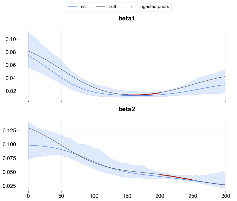
As seen above, for the ingested prior time window, the estimation is aligned better with the truth and the resulting confidence interval also becomes narrower compared to other periods.
References
Ng, Wang and Dai (2021). Bayesian Time Varying Coefficient Model with Applications to Marketing Mix Modeling, arXiv preprint arXiv:2106.03322