Build Your Own Model

One important feature of orbit is to allow developers to build their own models in a relatively flexible manner to serve their own purpose. This tutorial will go over a demo on how to build up a simple Bayesian linear regression model using Pyro API in the backend with orbit interface.

Orbit Class Design

In version 1.1.0, the classes within Orbit are re-designed as such:

1. Forecaster

2. Model

3. Estimator

Forecaster

Forecaster provides general interface for users to perform fit and predict task. It is further inherited to provide different types of forecasting methodology:

1. Maximum a posterior (MAP)

2. [Stochastic Variational Inference (SVI)]

3. Full Bayesian

The discrepancy on these three methods mainly lie on the posteriors estimation where MAP will yield point posterior estimate and can be extracted through the method get_point_posterior(). Meanwhile, SVI and Full Bayesian allow posterior sample extraction through the method get_posteriors(). Alternatively, you can also approximate point estimate by passing through additional arg such as point_method='median' in the .fit() process.

To make use of a Forecaster, one must provide these two objects:

1. Model

2. Estimator

Theses two objects are prototyped as abstract and next subsections will cover how they work.

Model

Model is an object defined by a class inherited from BaseTemplate a.k.a Model Template in the diagram below. It mainly turns the logic of fit() and predict() concrete by supplying the fitter as a file (PyStan) or a callable class (Pyro) and the internal predict() method. This object defines the overall inputs, model structure, parameters and likelihoods.

Estimator

Meanwhile, there are different APIs implement slightly different ways of sampling and optimization (for MAP). orbit is designed to support various APIs such as PyStan and Pyro (hopefully PyMC3, Numpyro in the future!). The logic separating the call of different APIs with different interface is done by the Estimator class which is further inherited in PyroEstimator and StanEstimator.

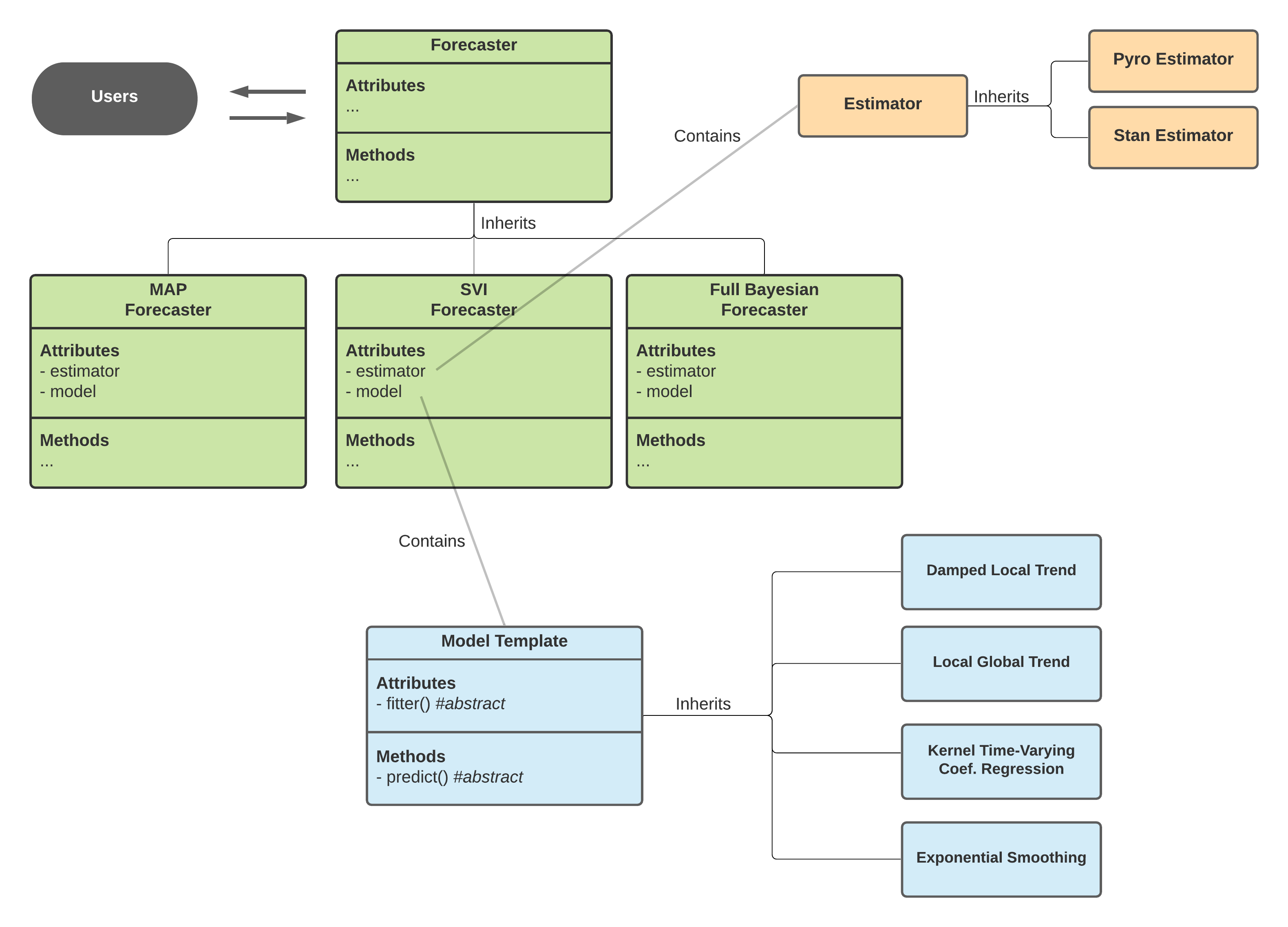
Diagram above shows the interaction across classes under the Orbit package design.

Creating a Bayesian Linear Regression Model

The plan here is to build a classical regression model with the formula below:

\[y = \alpha + X \beta + \epsilon\]

where \(\alpha\) is the intercept, \(\beta\) is the coefficients matrix and \(\epsilon\) is the random noise.

To start with let’s load the libraries.

import pandas as pd
import numpy as np
import torch
import pyro
import pyro.distributions as dist
from copy import deepcopy
import matplotlib.pyplot as plt

import orbit
from orbit.template.model_template import ModelTemplate
from orbit.forecaster import SVIForecaster
from orbit.estimators.pyro_estimator import PyroEstimatorSVI

from orbit.utils.simulation import make_regression
from orbit.diagnostics.plot import plot_predicted_data
from orbit.utils.plot import get_orbit_style
plt.style.use(get_orbit_style())

%matplotlib inline

print(orbit.__version__)

1.1.4

Since the Forecaster and Estimator are already built inside orbit, the rest of the ingredients to construct a new model will be a Model object that contains the follow:

• a callable class as a fitter

• a predict method

Define a Fitter

For Pyro users, you should find the code below familiar. All it does is to put a Bayesian linear regression (BLR) model code in a callable class. Details of BLR will not be covered here. Note that the parameters here need to be consistent .

class MyFitter:
    max_plate_nesting = 1  # max number of plates nested in model

    def __init__(self, data):
        for key, value in data.items():
            key = key.lower()
            if isinstance(value, (list, np.ndarray)):
                value = torch.tensor(value, dtype=torch.float)
            self.__dict__[key] = value

    def __call__(self):
        extra_out = {}

        p = self.regressor.shape[1]
        bias = pyro.sample("bias", dist.Normal(0, 1))
        weight = pyro.sample("weight", dist.Normal(0, 1).expand([p]).to_event(1))
        yhat = bias + weight @ self.regressor.transpose(-1, -2)
        obs_sigma = pyro.sample("obs_sigma", dist.HalfCauchy(self.response_sd))

        with pyro.plate("response_plate", self.num_of_obs):
            pyro.sample("response", dist.Normal(yhat, obs_sigma), obs=self.response)

        log_prob = dist.Normal(yhat[..., 1:], obs_sigma).log_prob(self.response[1:])
        extra_out.update(
            {"log_prob": log_prob}
        )

        return extra_out

Define the Model Class

This is the part requires the knowledge of orbit most. First we construct a class by plugging in the fitter callable. Users need to let the orbit estimators know the required input in addition to the defaults (e.g. response, response_sd etc.). In this case, it takes regressor as the matrix input from the data frame. That is why there are lines of code to provide this information in

1. _data_input_mapper - a list or Enum to let estimator keep tracking required data input

2. set_dynamic_attributes - the logic define the actual inputs i.e. regressor from the data frame. This is a reserved function being called inside Forecaster.

Finally, we code the logic in predict() to define how we utilize posteriors to perform in-sample / out-of-sample prediction. Note that the output needs to be a dictionary where it supports components decomposition.

class BayesLinearRegression(ModelTemplate):
    _fitter = MyFitter
    _data_input_mapper = ['regressor']
    _supported_estimator_types = [PyroEstimatorSVI]

    def __init__(self, regressor_col, **kwargs):
        super().__init__(**kwargs)
        self.regressor_col = regressor_col
        self.regressor = None
        self._model_param_names = ['bias', 'weight', 'obs_sigma']

    def set_dynamic_attributes(self, df, training_meta):
        self.regressor = df[self.regressor_col].values

    def predict(self, posterior_estimates, df, training_meta, prediction_meta, include_error=False, **kwargs):
        model = deepcopy(posterior_estimates)
        new_regressor = df[self.regressor_col].values.T
        bias =  np.expand_dims(model.get('bias'),-1)
        obs_sigma = np.expand_dims(model.get('obs_sigma'), -1)
        weight = model.get('weight')

        pred_len = df.shape[0]
        batch_size = weight.shape[0]

        prediction = bias + np.matmul(weight, new_regressor) + \
            np.random.normal(0, obs_sigma, size=(batch_size, pred_len))
        return {'prediction': prediction}

Test the New Model with Forecaster

Once the model class is defined. User can initialize an object and build a forecaster for fit and predict purpose. Before doing that, the demo provides a simulated dataset here.

Data Simulation

x, y, coefs = make_regression(120, [3.0, -1.0], bias=1.0, scale=1.0)

df = pd.DataFrame(
    np.concatenate([y.reshape(-1, 1), x], axis=1), columns=['y', 'x1', 'x2']
)
df['week'] = pd.date_range(start='2016-01-04', periods=len(y), freq='7D')

df.head(5)

	y	x1	x2	week
0	2.382337	0.345584	0.000000	2016-01-04
1	2.812929	0.330437	-0.000000	2016-01-11
2	3.600130	0.905356	0.446375	2016-01-18
3	-0.884275	-0.000000	0.581118	2016-01-25
4	2.704941	0.364572	0.294132	2016-02-01

test_size = 20
train_df = df[:-test_size]
test_df = df[-test_size:]

Create the Forecaster

As mentioned previously, model is the inner object to control the math. To use it for fit and predict purpose, we need a Forecaster. Since the model is written in Pyro, the pick here should be SVIForecaster.

model = BayesLinearRegression(
    regressor_col=['x1','x2'],
)

blr = SVIForecaster(
    model=model,
    response_col='y',
    date_col='week',
    estimator_type=PyroEstimatorSVI,
    verbose=True,
    num_steps=501,
    seed=2021,
)

blr

<orbit.forecaster.svi.SVIForecaster at 0x29ba8d4f0>

Now, an object blr is instantiated as a SVIForecaster object and is ready for fit and predict.

blr.fit(train_df)

<orbit.forecaster.svi.SVIForecaster at 0x29ba8d4f0>

Compare Coefficients with Truth

estimated_weights = blr.get_posterior_samples()['weight']

The code below is to compare the median of coefficients posteriors which is labeled as weight with the truth.

print("True Coef: {:.3f}, {:.3f}".format(coefs[0], coefs[1]) )
estimated_coef = np.median(estimated_weights, axis=0)
print("Estimated Coef: {:.3f}, {:.3f}".format(estimated_coef[0], estimated_coef[1]))

True Coef: 3.000, -1.000
Estimated Coef: 2.988, -0.958

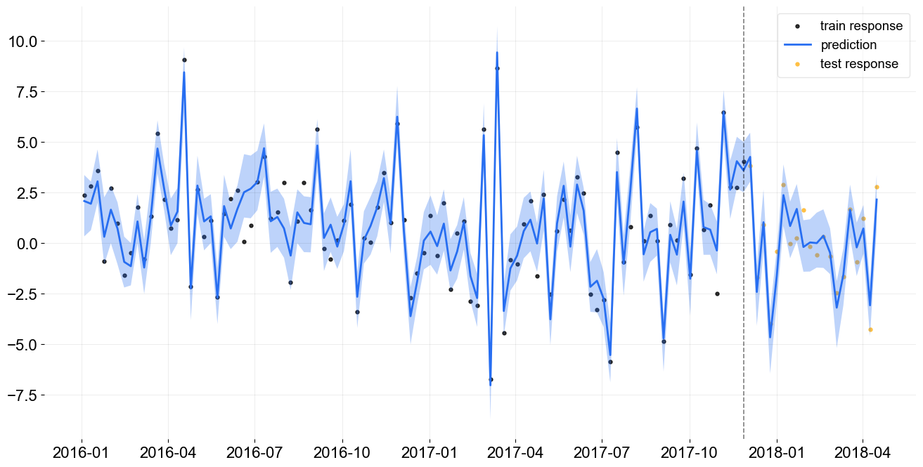
Examine Forecast Accuracy

predicted_df = blr.predict(df)

_ = plot_predicted_data(train_df, predicted_df, 'week', 'y', test_actual_df=test_df, prediction_percentiles=[5, 95])

Additional Notes

In general, most of the diagnostic tools in orbit such as posteriors checking and plotting is applicable in the model created in this style. Also, users can provide point_method='median' in the fit() under the SVIForecaster to extract median of posteriors directly.