Simulation Data

Orbit provide the functions to generate the simulation data including:

1. Generate the data with time-series trend:

   • random walk

   • arima

2. Generate the data with seasonality

   • discrete

   • fourier series

3. Generate regression data

import numpy as np
import matplotlib.pyplot as plt

import orbit
from orbit.utils.simulation import make_trend, make_seasonality, make_regression
from orbit.utils.plot import get_orbit_style
plt.style.use(get_orbit_style())
from orbit.constants.palette import OrbitPalette

%matplotlib inline

print(orbit.__version__)

1.1.4.6

Trend

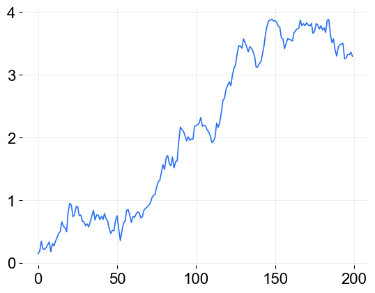
Random Walk

rw = make_trend(200, rw_loc=0.02, rw_scale=0.1, seed=2020)
_ = plt.plot(rw, color = OrbitPalette.BLUE.value)

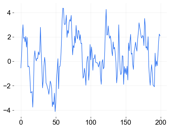
ARMA

reference for the ARMA process: https://www.statsmodels.org/stable/generated/statsmodels.tsa.arima_process.ArmaProcess.html

arma_trend =  make_trend(200, method='arma', arma=[.8, -.1], seed=2020)
_ = plt.plot(arma_trend, color = OrbitPalette.BLUE.value)

Seasonality

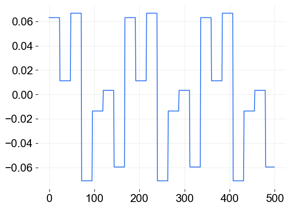
Discrete

generating a weekly seasonality(=7) where seasonality within a day is constant(duration=24) on an hourly time-series

ds = make_seasonality(500, seasonality=7, duration=24, method='discrete', seed=2020)
_ = plt.plot(ds, color = OrbitPalette.BLUE.value)

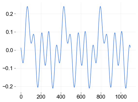
Fourier

generating a sine-cosine wave seasonality for a annual seasonality(=365) using fourier series

fs = make_seasonality(365 * 3, seasonality=365, method='fourier', order=5, seed=2020)
_ = plt.plot(fs, color = OrbitPalette.BLUE.value)

fs

array([0.01162034, 0.00739299, 0.00282248, ..., 0.02173615, 0.01883928,
       0.01545216])

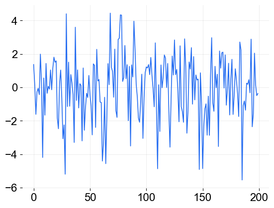
Regression

generating multiplicative time-series with trend, seasonality and regression components

# define the regression coefficients
coefs = [0.1, -.33, 0.8]

x, y, coefs = make_regression(200, coefs, scale=2.0, seed=2020)

_ = plt.plot(y, color = OrbitPalette.BLUE.value)

For next step, need to install scikit-learn

# !python -m pip install scikit-learn

from sklearn.linear_model import LinearRegression

# check if get the coefficients as set up
reg = LinearRegression().fit(x, y)
print(reg.coef_)

---------------------------------------------------------------------------
ModuleNotFoundError                       Traceback (most recent call last)
Cell In[12], line 1
----> 1 from sklearn.linear_model import LinearRegression
      3 # check if get the coefficients as set up 
      4 reg = LinearRegression().fit(x, y)

ModuleNotFoundError: No module named 'sklearn'