Local Global Trend (LGT)
In this section, we will cover:
LGT model structure
difference between DLT and LGT
syntax to call LGT classes with different estimation methods
LGT stands for Local and Global Trend and is a refined model from Rlgt (Smyl et al., 2019). The main difference is that LGT is an additive form taking log-transformation response as the modeling response. This essentially converts the model into a multiplicative with some advantages (Ng and Wang et al., 2020). However, one drawback of this approach is that negative response values are not allowed due to the existence of the global trend term and because of that we start to deprecate the support of regression of this model.
[1]:
%matplotlib inline

import pandas as pd
import numpy as np
import matplotlib.pyplot as plt

import orbit
from orbit.models import LGT
from orbit.diagnostics.plot import plot_predicted_data
from orbit.diagnostics.plot import plot_predicted_components
from orbit.utils.dataset import load_iclaims
[2]:
print(orbit.__version__)
1.1.4.6
Model Structure
with the update process,
Unlike DLT model which has a deterministic trend, LGT introduces a hybrid trend where it consists of
local trend takes on a fraction \(\xi_1\) rather than a damped factor
global trend is with a auto-regrssive term \(\xi_2\) and a power term \(\lambda\)
We will continue to use the iclaims data with 52 weeks train-test split.
[3]:
# load data
df = load_iclaims()
# define date and response column
date_col = 'week'
response_col = 'claims'
df.dtypes
test_size = 52
train_df = df[:-test_size]
test_df = df[-test_size:]
LGT Model
In orbit, we provide three methods for LGT model estimation and inferences, which are
MAP
MCMC (also providing the point estimate method,
meanormedian), which is also the defaultSVI
Orbit follows a sklearn style model API. We can create an instance of the Orbit class and then call its fit and predict methods.
In this notebook, we will only cover MAP and MCMC methods. Refer to this notebook for the pyro estimation.
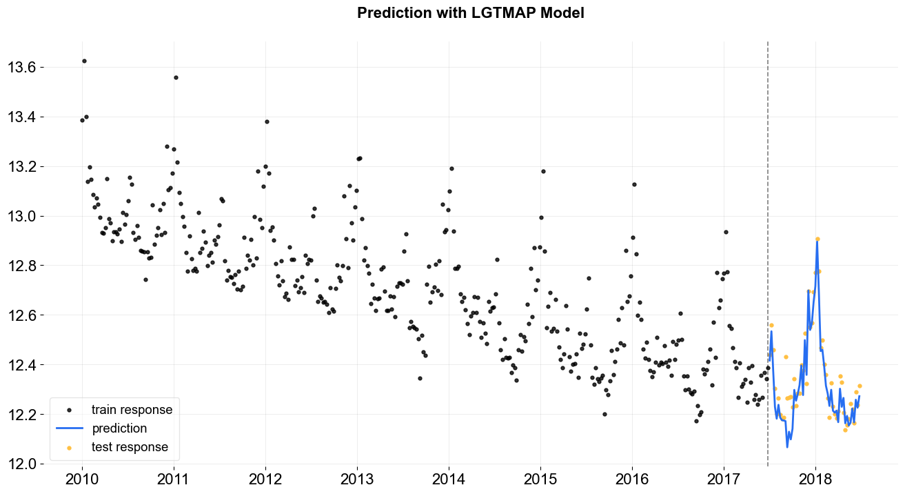
LGT - MAP
To use MAP, specify the estimator as stan-map.
[4]:
lgt = LGT(
    response_col=response_col,
    date_col=date_col,
    estimator='stan-map',
    seasonality=52,
    seed=8888,
)
2024-03-19 23:39:41 - orbit - INFO - Optimizing (CmdStanPy) with algorithm: LBFGS.
[5]:
%%time
lgt.fit(df=train_df)
CPU times: user 9.3 ms, sys: 16.8 ms, total: 26.1 ms
Wall time: 172 ms
[5]:
<orbit.forecaster.map.MAPForecaster at 0x2919dccd0>
[6]:
predicted_df = lgt.predict(df=test_df)
[7]:
_ = plot_predicted_data(training_actual_df=train_df, predicted_df=predicted_df,
                        date_col=date_col, actual_col=response_col,
                        test_actual_df=test_df, title='Prediction with LGTMAP Model')
LGT - MCMC
To use MCMC sampling, specify the estimator as stan-mcmc (the default).
By dedault, full Bayesian samples will be used for the predictions: for each set of parameter posterior samples, the prediction will be conducted once and the final predictions are aggregated over all the results. To be specific, the final predictions will be the median (aka 50th percentile) along with any additional percentiles provided. One can use
.get_posterior_samples()to extract the samples for all sampling parameters.One can also specify
point_method(eithermeanormedian) via.fitto have the point estimate: the parameter posterior samples are aggregated first (mean or median) then conduct the prediction once.
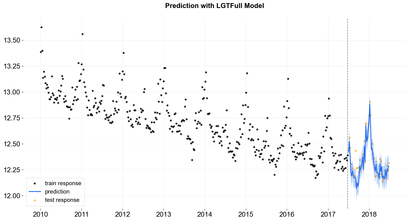
LGT - full
[8]:
lgt = LGT(
    response_col=response_col,
    date_col=date_col,
    seasonality=52,
    seed=2024,
    stan_mcmc_args={'show_progress': False},
)
[9]:
%%time
lgt.fit(df=train_df)
2024-03-19 23:39:42 - orbit - INFO - Sampling (CmdStanPy) with chains: 4, cores: 8, temperature: 1.000, warmups (per chain): 225 and samples(per chain): 25.
CPU times: user 87.1 ms, sys: 36.9 ms, total: 124 ms
Wall time: 5.13 s
[9]:
<orbit.forecaster.full_bayes.FullBayesianForecaster at 0x2a4bc4090>
[10]:
predicted_df = lgt.predict(df=test_df)
[11]:
predicted_df.tail(5)
[11]:
| week | prediction_5 | prediction | prediction_95 | |
|---|---|---|---|---|
| 47 | 2018-05-27 | 12.114602 | 12.250131 | 12.382320 |
| 48 | 2018-06-03 | 12.058250 | 12.173431 | 12.272940 |
| 49 | 2018-06-10 | 12.164898 | 12.253941 | 12.387880 |
| 50 | 2018-06-17 | 12.138711 | 12.241891 | 12.362063 |
| 51 | 2018-06-24 | 12.182641 | 12.284261 | 12.397172 |
[12]:
lgt.get_posterior_samples().keys()
[12]:
dict_keys(['l', 'b', 'lev_sm', 'slp_sm', 'obs_sigma', 'nu', 'lgt_sum', 'gt_pow', 'lt_coef', 'gt_coef', 's', 'sea_sm', 'loglk'])
[13]:
_ = plot_predicted_data(training_actual_df=train_df, predicted_df=predicted_df,
                    date_col=lgt.date_col, actual_col=lgt.response_col,
                    test_actual_df=test_df, title='Prediction with LGTFull Model')
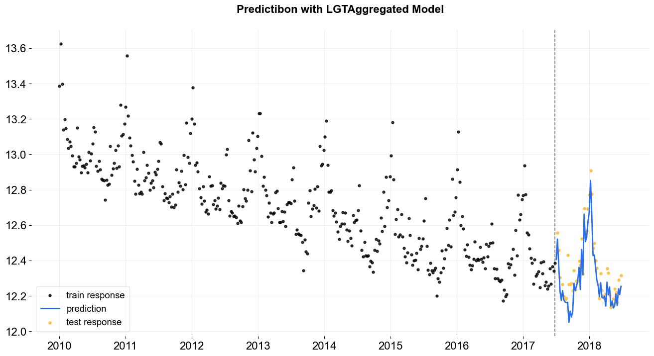
LGT - point estimate
[14]:
lgt = LGT(
    response_col=response_col,
    date_col=date_col,
    seasonality=52,
    seed=2024,
    stan_mcmc_args={'show_progress': False},
)
[15]:
%%time
lgt.fit(df=train_df, point_method='mean')
2024-03-19 23:39:47 - orbit - INFO - Sampling (CmdStanPy) with chains: 4, cores: 8, temperature: 1.000, warmups (per chain): 225 and samples(per chain): 25.
CPU times: user 97.2 ms, sys: 41.7 ms, total: 139 ms
Wall time: 4.64 s
[15]:
<orbit.forecaster.full_bayes.FullBayesianForecaster at 0x2a4d2add0>
[16]:
predicted_df = lgt.predict(df=test_df)
[17]:
predicted_df.tail(5)
[17]:
| week | prediction | |
|---|---|---|
| 47 | 2018-05-27 | 12.210257 |
| 48 | 2018-06-03 | 12.145213 |
| 49 | 2018-06-10 | 12.239412 |
| 50 | 2018-06-17 | 12.207138 |
| 51 | 2018-06-24 | 12.253422 |
[18]:
_ = plot_predicted_data(training_actual_df=train_df, predicted_df=predicted_df,
                    date_col=lgt.date_col, actual_col=lgt.response_col,
                    test_actual_df=test_df, title='Predictibon with LGTAggregated Model')