Regression Priors in DLT

This notebook demonstrates usage of priors in the regression analysis. The iclaims data will be used in demo purpose. Examples include

1. regression with default setting

2. regression with bounded priors for regression coefficients

Generally speaking, regression coefficients are more robust under full Bayesian sampling and estimation. The default setting estimator='stan-mcmc' will be used in this tutorial.

%matplotlib inline

import matplotlib.pyplot as plt
import numpy as np

import orbit
from orbit.utils.dataset import load_iclaims
from orbit.models import DLT
from orbit.diagnostics.plot import plot_predicted_data

print(orbit.__version__)

1.1.4.6

US Weekly Initial Claims

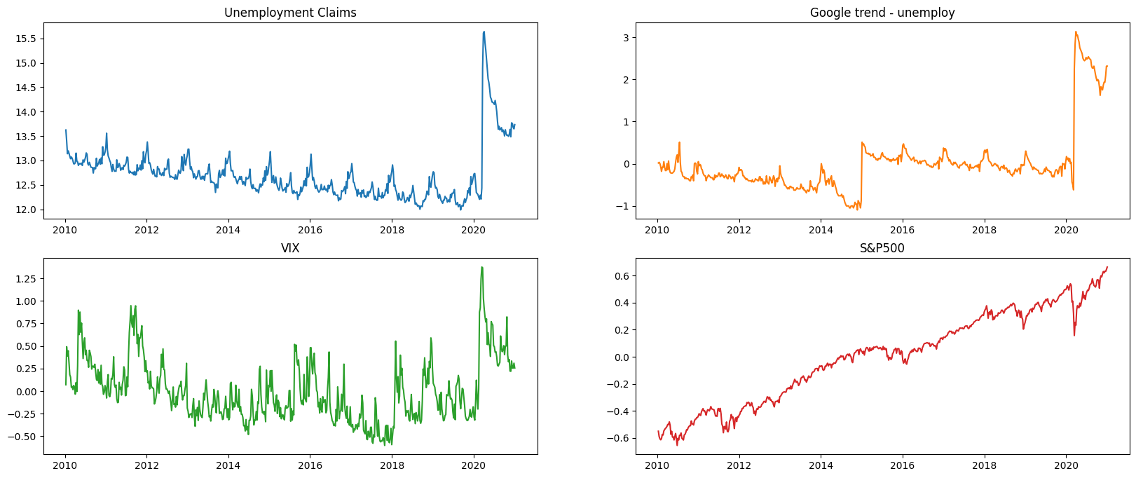
Recall the iclaims dataset by previous section. In order to use this data to nowcast the US unemployment claims during COVID-19 period, the dataset is extended to Jan 2021 and the S&P 500 (^GSPC) and VIX Index historical data are attached for the same period.

The data is standardized and log-transformed for the model fitting purpose.

# load data
df = load_iclaims(end_date='2021-01-03')
df = df[['week', 'claims', 'trend.unemploy', 'trend.job', 'sp500', 'vix']]
df = df[1:].reset_index(drop=True)

date_col = 'week'
response_col = 'claims'
df.dtypes

week              datetime64[ns]
claims                   float64
trend.unemploy           float64
trend.job                float64
sp500                    float64
vix                      float64
dtype: object

df.head(5)

	week	claims	trend.unemploy	trend.job	sp500	vix
0	2010-01-10	13.624218	0.016351	0.181862	-0.550891	0.069878
1	2010-01-17	13.398741	0.032611	0.130569	-0.590640	0.491772
2	2010-01-24	13.137549	-0.000179	0.119987	-0.607162	0.388078
3	2010-01-31	13.196760	-0.069172	0.087552	-0.614339	0.446838
4	2010-02-07	13.146984	-0.182500	0.019344	-0.605636	0.308205

We can see form the plot below, there are seasonality, trend, and as well as a huge change point due the impact of COVID-19.

fig, axs = plt.subplots(2, 2,figsize=(20,8))
axs[0, 0].plot(df['week'], df['claims'])
axs[0, 0].set_title('Unemployment Claims')
axs[0, 1].plot(df['week'], df['trend.unemploy'], 'tab:orange')
axs[0, 1].set_title('Google trend - unemploy')
axs[1, 0].plot(df['week'], df['vix'], 'tab:green')
axs[1, 0].set_title('VIX')
axs[1, 1].plot(df['week'], df['sp500'], 'tab:red')
axs[1, 1].set_title('S&P500')

Text(0.5, 1.0, 'S&P500')

# using relatively updated data
df[['sp500']] = df[['sp500']].diff()
df = df[1:].reset_index(drop=True)

test_size = 12
train_df = df[:-test_size]
test_df = df[-test_size:]

Naive Model

Here we will use DLT models to compare the model performance with vs. without regression.

%%time
dlt = DLT(
    response_col=response_col,
    date_col=date_col,
    seasonality=52,
    seed=8888,
    num_warmup=4000,
    stan_mcmc_args={'show_progress': False}
)
dlt.fit(df=train_df)
predicted_df = dlt.predict(df=test_df)

2024-03-19 23:42:14 - orbit - INFO - Sampling (CmdStanPy) with chains: 4, cores: 8, temperature: 1.000, warmups (per chain): 1000 and samples(per chain): 25.

CPU times: user 126 ms, sys: 39.3 ms, total: 165 ms
Wall time: 11 s

DLT With Regression

The regressor columns can be supplied via argument regressor_col. Recall the regression formula in DLT:

\[\begin{split}\hat{y}_t =\mu_t + s_t + r_t \\ r_t = \sum_{j}\beta_j x_{jt} \\ \beta_j ~\sim \mathcal{N}(\mu_j, \sigma_j^2)\end{split}\]

By default, \(\mu_j = 0\) and \(\sigma_j = 1\). In addition, we can set a sign constraint for each coefficient \(\beta_j\). This is can be done by supplying the regressor_sign as a list where elements are in one of followings:

• ‘=’: \(\beta_j ~\sim \mathcal{N}(0, \sigma_j^2)\) i.e. \(\beta_j \in (-\inf, \inf)\)

• ‘+’: \(\beta_j ~\sim \mathcal{N}^+(0, \sigma_j^2)\) i.e. \(\beta_j \in [0, \inf)\)

• ‘-’: \(\beta_j ~\sim \mathcal{N}^-(0, \sigma_j^2)\) i.e. \(\beta_j \in (-\inf, 0]\)

Based on some intuition, it’s reasonable to assume search terms such as “unemployment”, “filling” and VIX index to be positively correlated and stock index such as SP500 to be negatively correlated to the outcome. Then we will leave whatever unspecified as a regular regressor.

%%time
dlt_reg = DLT(
    response_col=response_col,
    date_col=date_col,
    regressor_col=['trend.unemploy', 'trend.job', 'sp500', 'vix'],
    seasonality=52,
    seed=8888,
    num_warmup=4000,
    stan_mcmc_args={'show_progress': False}
)
dlt_reg.fit(df=train_df)
predicted_df_reg = dlt_reg.predict(test_df)

2024-03-19 23:42:26 - orbit - INFO - Sampling (CmdStanPy) with chains: 4, cores: 8, temperature: 1.000, warmups (per chain): 1000 and samples(per chain): 25.

CPU times: user 164 ms, sys: 71.3 ms, total: 235 ms
Wall time: 13.3 s

The estimated regressor coefficients can be retrieved via .get_regression_coefs().

dlt_reg.get_regression_coefs()

	regressor	regressor_sign	coefficient	coefficient_lower	coefficient_upper	Pr(coef >= 0)	Pr(coef < 0)
0	trend.unemploy	Regular	0.076715	0.042656	0.105937	1.00	0.00
1	trend.job	Regular	-0.038551	-0.081939	0.019654	0.13	0.87
2	sp500	Regular	-0.001387	-0.201171	0.195193	0.49	0.51
3	vix	Regular	0.011533	-0.013659	0.035988	0.73	0.27

Regression with Informative Priors

Due to various reasons, users may obtain further knowledge on some of the regressors or they want to propose different regularization on different regressors. These informative priors basically means to replace the defaults (\(\mu\), \(\sigma\)) mentioned previously. In orbit, this process is done via the arguments regressor_beta_prior and regressor_sigma_prior. These two lists should be of the same length as regressor_col.

In addition, we can set a sign constraint for each coefficient \(\beta_j\). This is can be done by supplying the regressor_sign as a list where elements are in one of followings:

• ‘=’: \(\beta_j ~\sim \mathcal{N}(0, \sigma_j^2)\) i.e. \(\beta_j \in (-\inf, \inf)\)

• ‘+’: \(\beta_j ~\sim \mathcal{N}^+(0, \sigma_j^2)\) i.e. \(\beta_j \in [0, \inf)\)

• ‘-’: \(\beta_j ~\sim \mathcal{N}^-(0, \sigma_j^2)\) i.e. \(\beta_j \in (-\inf, 0]\)

Based on intuition, it’s reasonable to assume search terms such as “unemployment”, “filling” and VIX index to be positively correlated (+ sign is used in this case) and upward shock of SP500 (- sign) to be negatively correlated to the outcome. Otherwise, an unbounded coefficient can be used (= sign).

Furthermore, regressors such as search queries may have more direct impact than stock marker indices. Hence, a smaller \(\sigma\) is considered.

dlt_reg_adjust = DLT(
    response_col=response_col,
    date_col=date_col,
    regressor_col=['trend.unemploy', 'trend.job', 'sp500','vix'],
    regressor_sign=['+','=','-','+'],
    regressor_sigma_prior=[0.3, 0.1, 0.05, 0.1],
    num_warmup=4000,
    num_sample=1000,
    estimator='stan-mcmc',
    seed=2022,
    stan_mcmc_args={'show_progress': False}
)
dlt_reg_adjust.fit(df=train_df)
predicted_df_reg_adjust = dlt_reg_adjust.predict(test_df)

2024-03-19 23:42:39 - orbit - INFO - Sampling (CmdStanPy) with chains: 4, cores: 8, temperature: 1.000, warmups (per chain): 1000 and samples(per chain): 250.

dlt_reg_adjust.get_regression_coefs()

	regressor	regressor_sign	coefficient	coefficient_lower	coefficient_upper	Pr(coef >= 0)	Pr(coef < 0)
0	trend.unemploy	Positive	0.126584	0.075630	0.198016	1.000	0.000
1	vix	Positive	0.019553	0.002202	0.054368	1.000	0.000
2	sp500	Negative	-0.032251	-0.087838	-0.002386	0.000	1.000
3	trend.job	Regular	-0.011294	-0.086100	0.058422	0.394	0.606

Let’s compare the holdout performance by using the built-in function smape() .

def mae(x, y):
    return np.mean(np.abs(x - y))

naive_mae = mae(predicted_df['prediction'].values, test_df['claims'].values)
reg_mae = mae(predicted_df_reg['prediction'].values, test_df['claims'].values)
reg_adjust_mae = mae(predicted_df_reg_adjust['prediction'].values, test_df['claims'].values)

print("----------------Mean Absolute Error Summary----------------")
print("Naive Model: {:.3f}\nRegression Model: {:.3f}\nRefined Regression Model: {:.3f}".format(
    naive_mae, reg_mae, reg_adjust_mae
))

----------------Mean Absolute Error Summary----------------
Naive Model: 0.255
Regression Model: 0.242
Refined Regression Model: 0.096

Summary

This demo showcases a use case in nowcasting. Although this may not be applicable in real-time forecasting, it mainly introduces the regression analysis with time-series modeling in Orbit. For people who have concerns on the forecastability, one can consider introducing lag on regressors.

Also, Orbit allows informative priors where sometime can be useful in combining multiple source of insights together.