Kernel-based Time-varying Regression - Part II
The previous tutorial covered the basic syntax and structure of KTR (or so called BTVC); time-series data was fitted with a KTR model accounting for trend and seasonality. In this tutorial a KTR model is fit with trend, seasonality, and additional regressors. To summarize part 1, KTR considers a time-series as an additive combination of local-trend, seasonality, and additional regressors. The coefficients for all three components are allowed to vary over time. The time-varying of the coefficients is modeled using kernel smoothing of latent variables. This can also be an advantage of picking this model over other static regression coefficients models.
This tutorial covers:
KTR model structure with regression
syntax to initialize, fit and predict a model with regressors
visualization of regression coefficients
[1]:
import pandas as pd
import numpy as np
from math import pi
import matplotlib.pyplot as plt

import orbit
from orbit.models import KTR
from orbit.diagnostics.plot import plot_predicted_components
from orbit.utils.plot import get_orbit_style
from orbit.constants.palette import OrbitPalette

%matplotlib inline
pd.set_option('display.float_format', lambda x: '%.5f' % x)
orbit_style = get_orbit_style()
plt.style.use(orbit_style);
[2]:
print(orbit.__version__)
1.1.4.6
Model Structure
This section gives the mathematical structure of the KTR model. In short, it considers a time-series (\(y_t\)) as the linear combination of three parts. These are the local-trend (\(l_t\)), seasonality (s_t), and regression (\(r_t\)) terms at time \(t\). That is
where
\(\epsilon_t\)s comprise a stationary random error process.
\(r_t\) is the regression component which can be further expressed as \(\sum_{i=1}^{I} {x_{i,t}\beta_{i, t}}\) with covariate \(x\) and coefficient \(\beta\) on indexes \(i,t\)
For details of how on \(l_t\) and \(s_t\), please refer to Part I.
Recall in KTR, we express coefficients as
where
coefficient matrix \(\text{B}\) has size \(t \times P\) with rows equal to the \(\beta_t\)
knot matrix \(b\) with size \(P\times J\); each entry is a latent variable \(b_{p, j}\). The \(b_j\) can be viewed as the “knots” from the perspective of spline regression and \(j\) is a time index such that \(t_j \in [1, \cdots, T]\).
kernel matrix \(K\) with size \(T\times J\) where the \(i\)th row and \(j\)th element can be viewed as the normalized weight \(k(t_j, t) / \sum_{j=1}^{J} k(t_j, t)\)
In regression, we generate the matrix \(K\) with Gaussian kernel \(k_\text{reg}\) as such:
\(k_\text{reg}(t, t_j;\rho) = \exp ( -\frac{(t-t_j)^2}{2\rho^2} ),\)
where \(\rho\) is the scale hyper-parameter.
Data Simulation Module
In this example, we will use simulated data in order to have true regression coefficients for comparison. We propose two set of simulation data with three predictors each:
The two data sets are:
random walk
sine-cosine like
Note the data are random so it may be worthwhile to repeat the next few sets a few times to see how different data sets work.
Random Walk Simulated Dataset
[3]:
def sim_data_seasonal(n, RS):
    """ coefficients curve are sine-cosine like
    """
    np.random.seed(RS)
    # make the time varing coefs
    tau = np.arange(1, n+1)/n
    data = pd.DataFrame({
        'tau': tau,
        'date': pd.date_range(start='1/1/2018', periods=n),
        'beta1': 2 * tau,
        'beta2': 1.01 + np.sin(2*pi*tau),
        'beta3': 1.01 + np.sin(4*pi*(tau-1/8)),
        'x1': np.random.normal(0, 10, size=n),
        'x2': np.random.normal(0, 10, size=n),
        'x3': np.random.normal(0, 10, size=n),
        'trend': np.cumsum(np.concatenate((np.array([1]), np.random.normal(0, 0.1, n-1)))),
        'error': np.random.normal(0, 1, size=n) #stats.t.rvs(30, size=n),#
    })

    data['y'] = data.x1 * data.beta1 + data.x2 * data.beta2 + data.x3 * data.beta3 + data.error
    return data
[4]:
def sim_data_rw(n, RS, p=3):
    """ coefficients curve are random walk like
    """
    np.random.seed(RS)

    # initializing coefficients at zeros, simulate all coefficient values
    lev = np.cumsum(np.concatenate((np.array([5.0]), np.random.normal(0, 0.01, n-1))))
    beta = np.concatenate(
        [np.random.uniform(0.05, 0.12, size=(1,p)),
         np.random.normal(0.0, 0.01, size=(n-1,p))],
            axis=0)
    beta = np.cumsum(beta, 0)

    # simulate regressors
    covariates = np.random.normal(0, 10, (n, p))

    # observation with noise
    y = lev + (covariates * beta).sum(-1) + 0.3 * np.random.normal(0, 1, n)

    regressor_col = ['x{}'.format(pp) for pp in range(1, p+1)]
    data = pd.DataFrame(covariates, columns=regressor_col)
    beta_col = ['beta{}'.format(pp) for pp in range(1, p+1)]
    beta_data = pd.DataFrame(beta, columns=beta_col)
    data = pd.concat([data, beta_data], axis=1)

    data['y'] = y
    data['date'] = pd.date_range(start='1/1/2018', periods=len(y))

    return data
[5]:
rw_data = sim_data_rw(n=300, RS=2021, p=3)
rw_data.head(10)
[5]:
| x1 | x2 | x3 | beta1 | beta2 | beta3 | y | date | |
|---|---|---|---|---|---|---|---|---|
| 0 | 14.02970 | -2.55469 | 4.93759 | 0.07288 | 0.06251 | 0.09662 | 6.11704 | 2018-01-01 |
| 1 | 6.23970 | 0.57014 | -6.99700 | 0.06669 | 0.05440 | 0.10476 | 5.35784 | 2018-01-02 |
| 2 | 9.91810 | -6.68728 | -3.68957 | 0.06755 | 0.04487 | 0.11624 | 4.82567 | 2018-01-03 |
| 3 | -1.17724 | 8.88090 | -16.02765 | 0.05849 | 0.04305 | 0.12294 | 3.63605 | 2018-01-04 |
| 4 | 11.61065 | 1.95306 | 0.19901 | 0.06604 | 0.03281 | 0.11897 | 5.85913 | 2018-01-05 |
| 5 | 7.31929 | 3.36017 | -6.09933 | 0.07825 | 0.03448 | 0.10836 | 5.08805 | 2018-01-06 |
| 6 | 0.53405 | 8.80412 | -1.83692 | 0.07467 | 0.01847 | 0.10507 | 4.59303 | 2018-01-07 |
| 7 | -16.03947 | 0.27562 | -22.00964 | 0.06887 | 0.00865 | 0.10749 | 1.26651 | 2018-01-08 |
| 8 | -17.72238 | 2.65195 | 0.22571 | 0.07007 | 0.01008 | 0.10432 | 4.10629 | 2018-01-09 |
| 9 | -7.39895 | -7.63162 | 3.25535 | 0.07715 | 0.01498 | 0.09356 | 4.30788 | 2018-01-10 |
Sine-Cosine Like Simulated Dataset
[6]:
sc_data = sim_data_seasonal(n=80, RS=2021)
sc_data.head(10)
[6]:
| tau | date | beta1 | beta2 | beta3 | x1 | x2 | x3 | trend | error | y | |
|---|---|---|---|---|---|---|---|---|---|---|---|
| 0 | 0.01250 | 2018-01-01 | 0.02500 | 1.08846 | 0.02231 | 14.88609 | 1.56556 | -14.69399 | 1.00000 | -0.73476 | 1.01359 |
| 1 | 0.02500 | 2018-01-02 | 0.05000 | 1.16643 | 0.05894 | 6.76011 | -0.56861 | 4.93157 | 1.07746 | -0.97007 | -1.00463 |
| 2 | 0.03750 | 2018-01-03 | 0.07500 | 1.24345 | 0.11899 | -4.18451 | -5.38234 | -13.90578 | 1.19201 | -0.13891 | -8.80009 |
| 3 | 0.05000 | 2018-01-04 | 0.10000 | 1.31902 | 0.20098 | -8.06521 | 9.01387 | -0.75244 | 1.22883 | 0.66550 | 11.59721 |
| 4 | 0.06250 | 2018-01-05 | 0.12500 | 1.39268 | 0.30289 | 5.55876 | 2.24944 | -2.53510 | 1.31341 | -1.58259 | 1.47715 |
| 5 | 0.07500 | 2018-01-06 | 0.15000 | 1.46399 | 0.42221 | -7.05504 | 12.77788 | 14.25841 | 1.25911 | -0.98049 | 22.68806 |
| 6 | 0.08750 | 2018-01-07 | 0.17500 | 1.53250 | 0.55601 | 11.30858 | 6.29269 | 7.82098 | 1.23484 | -0.53751 | 15.43357 |
| 7 | 0.10000 | 2018-01-08 | 0.20000 | 1.59779 | 0.70098 | 6.45002 | 3.61891 | 16.28098 | 1.13237 | -1.32858 | 17.15636 |
| 8 | 0.11250 | 2018-01-09 | 0.22500 | 1.65945 | 0.85357 | 1.06414 | 36.38726 | 8.80457 | 1.02834 | 0.87859 | 69.01607 |
| 9 | 0.12500 | 2018-01-10 | 0.25000 | 1.71711 | 1.01000 | 4.22155 | -12.01221 | 8.43176 | 1.00649 | -0.22055 | -11.27534 |
Fitting a Model with Regressors
The metadata for simulated data sets.
[7]:
# num of predictors
p = 3
regressor_col = ['x{}'.format(pp) for pp in range(1, p + 1)]
response_col = 'y'
date_col='date'
As in Part I KTR follows sklearn model API style. First an instance of the Orbit class KTR is created. Second fit and predict methods are called for that instance. Besides providing meta data such response_col, date_col and regressor_col, there are additional args to provide to specify the estimator and the setting of the estimator. For details, please refer to other tutorials of the Orbit site.
[8]:
ktr = KTR(
    response_col=response_col,
    date_col=date_col,
    regressor_col=regressor_col,
    prediction_percentiles=[2.5, 97.5],
    seed=2021,
    estimator='pyro-svi',
)
Here predict has the additional argument decompose=True. This returns the compponents (\(l_t\), \(s_t\), and \(r_t\)) of the regression along with the prediction.
[9]:
ktr.fit(df=rw_data)
ktr.predict(df=rw_data, decompose=True).head(5)
2024-03-19 23:38:29 - orbit - INFO - Optimizing (CmdStanPy) with algorithm: LBFGS.
2024-03-19 23:38:29 - orbit - INFO - Using SVI (Pyro) with steps: 301, samples: 100, learning rate: 0.1, learning_rate_total_decay: 1.0 and particles: 100.
/Users/towinazure/opt/miniconda3/envs/orbit311/lib/python3.11/site-packages/torch/__init__.py:696: UserWarning: torch.set_default_tensor_type() is deprecated as of PyTorch 2.1, please use torch.set_default_dtype() and torch.set_default_device() as alternatives. (Triggered internally at /Users/runner/work/pytorch/pytorch/pytorch/torch/csrc/tensor/python_tensor.cpp:453.)
  _C._set_default_tensor_type(t)
2024-03-19 23:38:30 - orbit - INFO - step    0 loss = 3107.8, scale = 0.091353
INFO:orbit:step    0 loss = 3107.8, scale = 0.091353
2024-03-19 23:38:31 - orbit - INFO - step  100 loss = 307.18, scale = 0.04889
INFO:orbit:step  100 loss = 307.18, scale = 0.04889
2024-03-19 23:38:32 - orbit - INFO - step  200 loss = 299.24, scale = 0.052646
INFO:orbit:step  200 loss = 299.24, scale = 0.052646
2024-03-19 23:38:33 - orbit - INFO - step  300 loss = 314.51, scale = 0.05106
INFO:orbit:step  300 loss = 314.51, scale = 0.05106
[9]:
| date | prediction_2.5 | prediction | prediction_97.5 | trend_2.5 | trend | trend_97.5 | regression_2.5 | regression | regression_97.5 | |
|---|---|---|---|---|---|---|---|---|---|---|
| 0 | 2018-01-01 | 5.18593 | 6.31800 | 7.44407 | 4.01896 | 5.17107 | 6.39624 | 0.83381 | 1.13830 | 1.45459 |
| 1 | 2018-01-02 | 3.28170 | 4.32130 | 5.31726 | 4.10800 | 5.12472 | 6.16573 | -1.01967 | -0.81734 | -0.55723 |
| 2 | 2018-01-03 | 3.39199 | 4.60176 | 5.90753 | 4.06752 | 5.24010 | 6.53175 | -0.91607 | -0.61901 | -0.25905 |
| 3 | 2018-01-04 | 2.05339 | 3.21789 | 4.37279 | 3.99131 | 5.11851 | 6.26958 | -2.30892 | -1.89482 | -1.38973 |
| 4 | 2018-01-05 | 4.73718 | 5.65588 | 6.60197 | 4.14160 | 5.13381 | 6.08087 | 0.31028 | 0.55018 | 0.78230 |
Visualization of Regression Coefficient Curves
The function get_regression_coefs to extract coefficients (they will have central credibility intervals if the argument include_ci=True is used).
[10]:
coef_mid, coef_lower, coef_upper = ktr.get_regression_coefs(include_ci=True)
[11]:
coef_mid.head(5)
[11]:
| date | x1 | x2 | x3 | |
|---|---|---|---|---|
| 0 | 2018-01-01 | 0.03861 | 0.06444 | 0.15967 |
| 1 | 2018-01-02 | 0.03766 | 0.06358 | 0.15637 |
| 2 | 2018-01-03 | 0.03670 | 0.06271 | 0.15305 |
| 3 | 2018-01-04 | 0.03573 | 0.06182 | 0.14970 |
| 4 | 2018-01-05 | 0.03475 | 0.06092 | 0.14633 |
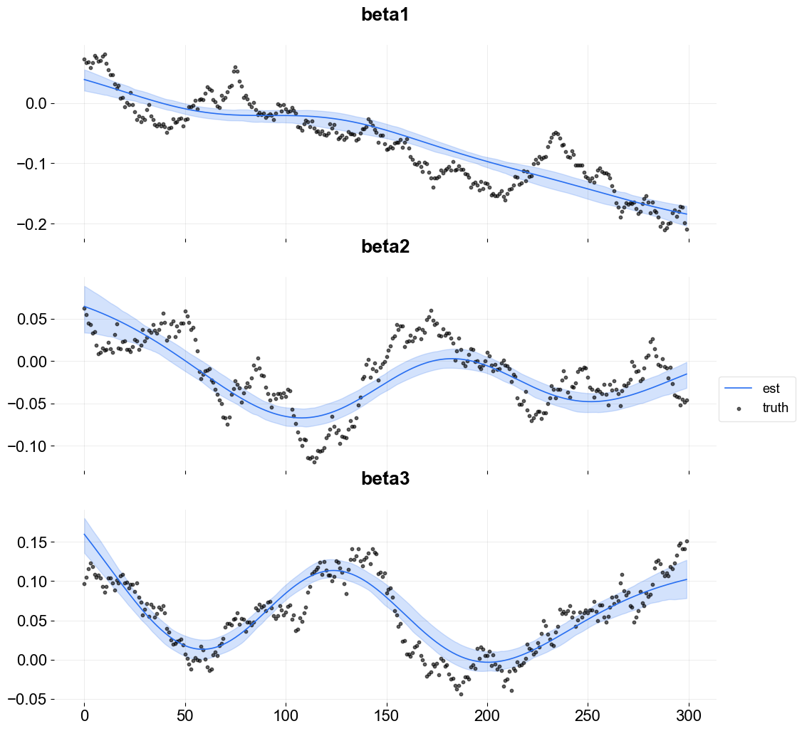
Because this is simulated data it is possible to overlay the estimate with the true coefficients.
[12]:
fig, axes = plt.subplots(p, 1, figsize=(12, 12), sharex=True)

x = np.arange(coef_mid.shape[0])
for idx in range(p):
    axes[idx].plot(x, coef_mid['x{}'.format(idx + 1)], label='est' if idx == 0 else "", color=OrbitPalette.BLUE.value)
    axes[idx].fill_between(x, coef_lower['x{}'.format(idx + 1)], coef_upper['x{}'.format(idx + 1)], alpha=0.2, color=OrbitPalette.BLUE.value)
    axes[idx].scatter(x, rw_data['beta{}'.format(idx + 1)], label='truth' if idx == 0 else "", s=10, alpha=0.6, color=OrbitPalette.BLACK.value)
    axes[idx].set_title('beta{}'.format(idx + 1))

fig.legend(bbox_to_anchor = (1,0.5));
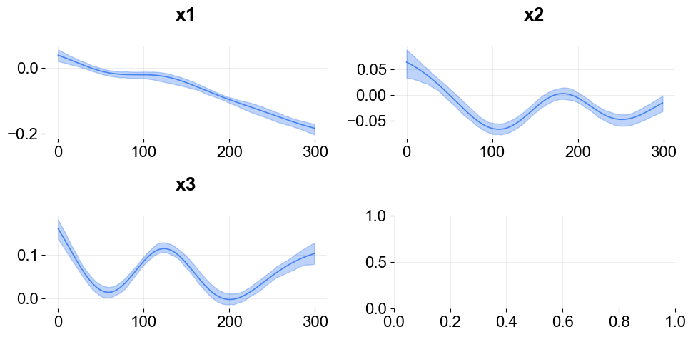
To plot coefficients use the function plot_regression_coefs from the KTR class.
[13]:
ktr.plot_regression_coefs(figsize=(10, 5), include_ci=True);
These type of time-varying coefficients detection problems are not new. Bayesian approach such as the R packages Bayesian Structural Time Series (a.k.a BSTS) by Scott and Varian (2014) and tvReg Isabel Casas and Ruben Fernandez-Casal (2021). Other frequentist approach such as Wu and Chiang (2000).
For further studies on benchmarking coefficients detection, Ng, Wang and Dai (2021) provides a detailed comparison of KTR with other popular time-varying coefficients methods; KTR demonstrates superior performance in the random walk data simulation.
Customizing Priors and Number of Knot Segments
To demonstrate how to specify the number of knots and priors consider the sine-cosine like simulated dataset. In this dataset, the fitting is more tricky since there could be some better way to define the number and position of the knots. There are obvious “change points” within the sine-cosine like curves. In KTR there are a few arguments that can leveraged to assign a priori knot attributes:
regressor_init_knot_locis used to define the prior mean of the knot value. e.g. in this case, there is not a lot of prior knowledge so zeros are used.The
regressor_init_knot_scaleandregressor_knot_scaleare used to tune the prior sd of the global mean of the knot and the sd of each knot from the global mean respectively. These create a plausible range for the knot values.The
regression_segmentsdefines the number of between knot segments (the number of knots - 1). The higher the number of segments the more change points are possible.
[14]:
ktr = KTR(
    response_col=response_col,
    date_col=date_col,

    regressor_col=regressor_col,
    regressor_init_knot_loc=[0] * len(regressor_col),
    regressor_init_knot_scale=[10.0] * len(regressor_col),
    regressor_knot_scale=[2.0] * len(regressor_col),
    regression_segments=6,

    prediction_percentiles=[2.5, 97.5],
    seed=2021,
    estimator='pyro-svi',
)
ktr.fit(df=sc_data)
2024-03-19 23:38:33 - orbit - INFO - Optimizing (CmdStanPy) with algorithm: LBFGS.
INFO:orbit:Optimizing (CmdStanPy) with algorithm: LBFGS.
2024-03-19 23:38:33 - orbit - INFO - Using SVI (Pyro) with steps: 301, samples: 100, learning rate: 0.1, learning_rate_total_decay: 1.0 and particles: 100.
INFO:orbit:Using SVI (Pyro) with steps: 301, samples: 100, learning rate: 0.1, learning_rate_total_decay: 1.0 and particles: 100.
2024-03-19 23:38:33 - orbit - INFO - step    0 loss = 828.02, scale = 0.10882
INFO:orbit:step    0 loss = 828.02, scale = 0.10882
2024-03-19 23:38:34 - orbit - INFO - step  100 loss = 340.58, scale = 0.87797
INFO:orbit:step  100 loss = 340.58, scale = 0.87797
2024-03-19 23:38:35 - orbit - INFO - step  200 loss = 266.67, scale = 0.37411
INFO:orbit:step  200 loss = 266.67, scale = 0.37411
2024-03-19 23:38:36 - orbit - INFO - step  300 loss = 261.21, scale = 0.43775
INFO:orbit:step  300 loss = 261.21, scale = 0.43775
[14]:
<orbit.forecaster.svi.SVIForecaster at 0x2b3ab0b10>
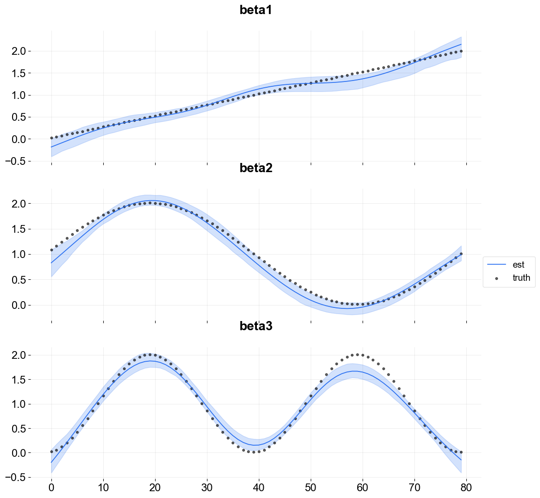
[15]:
coef_mid, coef_lower, coef_upper  = ktr.get_regression_coefs(include_ci=True)
fig, axes = plt.subplots(p, 1, figsize=(12, 12), sharex=True)

x = np.arange(coef_mid.shape[0])
for idx in range(p):
    axes[idx].plot(x, coef_mid['x{}'.format(idx + 1)], label='est' if idx == 0 else "", color=OrbitPalette.BLUE.value)
    axes[idx].fill_between(x, coef_lower['x{}'.format(idx + 1)], coef_upper['x{}'.format(idx + 1)], alpha=0.2, color=OrbitPalette.BLUE.value)
    axes[idx].scatter(x, sc_data['beta{}'.format(idx + 1)], label='truth' if idx == 0 else "", s=10, alpha=0.6, color=OrbitPalette.BLACK.value)
    axes[idx].set_title('beta{}'.format(idx + 1))

fig.legend(bbox_to_anchor = (1, 0.5));
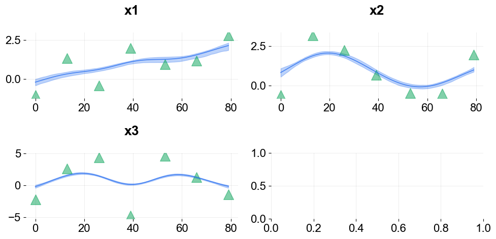
Visualize the knots using the plot_regression_coefs function with with_knot=True.
[16]:
ktr.plot_regression_coefs(with_knot=True, figsize=(10, 5), include_ci=True);
There are more ways to define knots for regression as well as seasonality and trend (a.k.a levels). These are described in Part III
References
Ng, Wang and Dai (2021). Bayesian Time Varying Coefficient Model with Applications to Marketing Mix Modeling, arXiv preprint arXiv:2106.03322
Isabel Casas and Ruben Fernandez-Casal (2021). tvReg: Time-Varying Coefficients Linear Regression for Single and Multi-Equations. https://CRAN.R-project.org/package=tvReg R package version 0.5.4.
Steven L Scott and Hal R Varian (2014). Predicting the present with bayesian structural time series. International Journal of Mathematical Modelling and Numerical Optimisation 5, 1-2 (2014), 4–23.