Methods of Estimations and Predictions
There are three methods supported in Orbit model parameters estimation (a.k.a posteriors in Bayesian).
Maximum a Posteriori (MAP)
Markov Chain Monte Carlo (MCMC)
Stochastic Variational Inference (SVI)
This session will cover the first two: MAP and MCMC which mainly uses CmdStanPy at the back end. Users can simply can leverage the args estimator to pick the method (stan-map and stan-mcmc). The details will be covered by the sections below. The SVI method is calling Pyro by specifying estimator='pyro-svi'. However, it is covered by a separate session.
Data and Libraries
[1]:
%matplotlib inline
import matplotlib.pyplot as plt

import orbit
from orbit.utils.dataset import load_iclaims
from orbit.models import ETS
from orbit.diagnostics.plot import plot_predicted_data, plot_predicted_components
[2]:
print(orbit.__version__)
1.1.4.6
[3]:
# load data
df = load_iclaims()
test_size = 52
train_df = df[:-test_size]
test_df = df[-test_size:]
response_col = 'claims'
date_col = 'week'
Maximum a Posteriori (MAP)
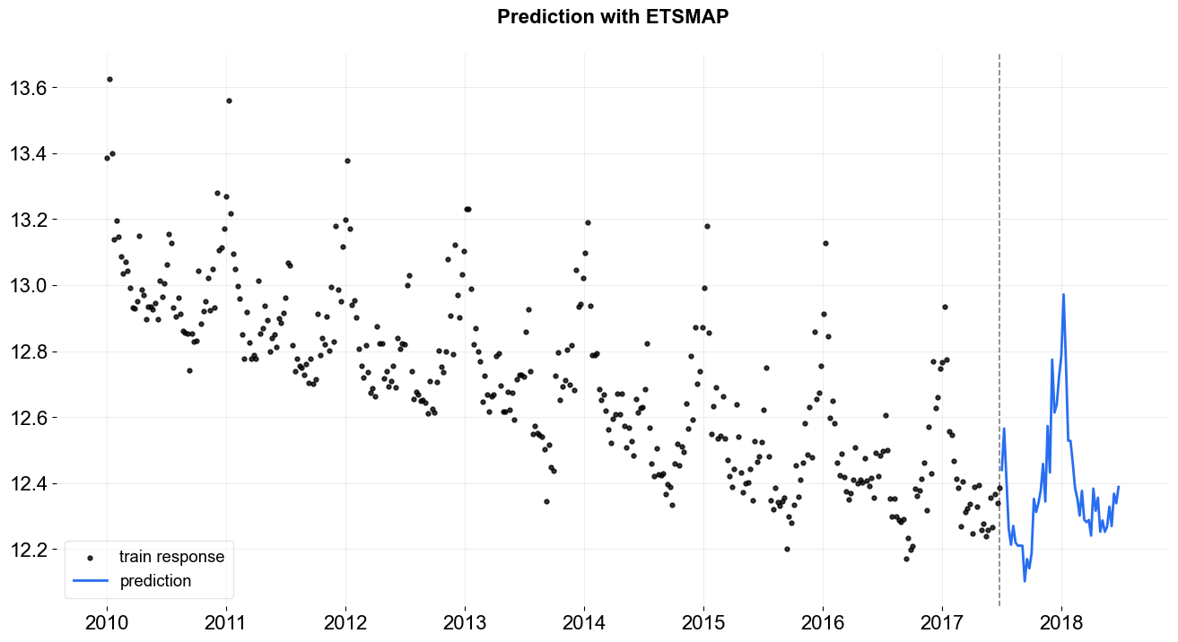
To use MAP method, one can simply specify estimator='stan-map' when instantiating a model. The advantage of MAP estimation is a faster computational speed. In MAP, the uncertainty is mainly generated the noise process with bootstrapping. However, the uncertainty would not cover parameters variance as well as the credible interval from seasonality or other components.
[4]:
%%time
ets = ETS(
    response_col=response_col,
    date_col=date_col,
    estimator='stan-map',
    seasonality=52,
    seed=8888,
)
ets.fit(df=train_df)
predicted_df = ets.predict(df=test_df)
2024-03-19 23:40:31 - orbit - INFO - Optimizing (CmdStanPy) with algorithm: LBFGS.
CPU times: user 9.55 ms, sys: 11.8 ms, total: 21.3 ms
Wall time: 75.3 ms
[5]:
_ = plot_predicted_data(train_df, predicted_df, date_col, response_col, title='Prediction with ETSMAP')
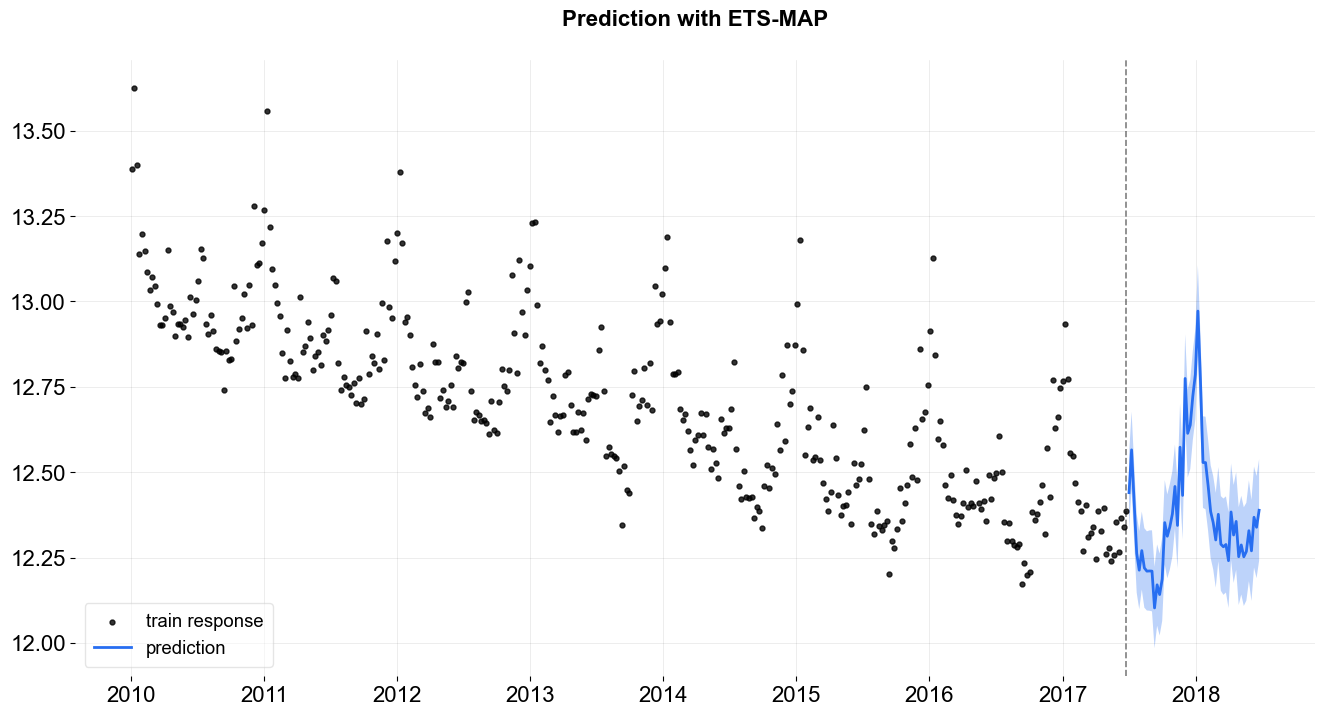
To have the uncertainty from MAP, one can speicify n_bootstrap_draws. The default is set to be -1 which mutes the bootstrap process. Users can also specify a particular percentiles to report prediction intervals by passing list of percentiles with args prediction_percentiles.
[6]:
# default: [10, 90]
prediction_percentiles=[10, 90]
ets = ETS(
    response_col=response_col,
    date_col=date_col,
    estimator='stan-map',
    seasonality=52,
    seed=8888,
    n_bootstrap_draws=1e4,
    prediction_percentiles=prediction_percentiles,
)
ets.fit(df=train_df)
predicted_df = ets.predict(df=test_df)

_ = plot_predicted_data(train_df, predicted_df, date_col, response_col,
                        prediction_percentiles=prediction_percentiles,
                        title='Prediction with ETS-MAP')
2024-03-19 23:40:32 - orbit - INFO - Optimizing (CmdStanPy) with algorithm: LBFGS.
One can access the posterior estimated by calling the .get_point_posteriors(). The outcome from this function is a dict of dict where the top layer stores the type of point estimate while the second layer stores the parameters labels and values.
[7]:
pt_posteriors = ets.get_point_posteriors()['map']
pt_posteriors.keys()
[7]:
dict_keys(['l', 'lev_sm', 'obs_sigma', 's', 'sea_sm'])
In general, the first dimension is just 1 as a point estimate for each parameter. The rest of the dimension will depend on the dimension of parameter itself.
[8]:
lev = pt_posteriors['l']
lev.shape
[8]:
(1, 391)
MCMC
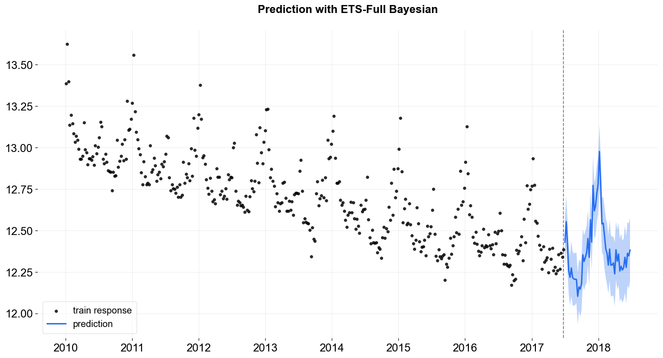
To use MCMC method, one can specify estimator='stan-mcmc' (the default) when instantiating a model. Compared to MAP, it usually takes longer time to fit. As the model now fitted as a full Bayesian model where No-U-Turn Sampler (NUTS) (Hoffman and Gelman 2011) is carried out under the hood. By default, a full sampling on posteriors distribution is conducted. Hence, full distribution of the predictions are always provided.
MCMC - Full Bayesian Sampling
[9]:
%%time
ets = ETS(
    response_col=response_col,
    date_col=date_col,
    estimator='stan-mcmc',
    seasonality=52,
    seed=8888,
    num_warmup=400,
    num_sample=400,
    stan_mcmc_args={'show_progress': False},
)
ets.fit(df=train_df)
predicted_df = ets.predict(df=test_df)
2024-03-19 23:40:32 - orbit - INFO - Sampling (CmdStanPy) with chains: 4, cores: 8, temperature: 1.000, warmups (per chain): 100 and samples(per chain): 100.
CPU times: user 143 ms, sys: 45.5 ms, total: 189 ms
Wall time: 608 ms
[10]:
_ = plot_predicted_data(train_df, predicted_df, date_col, response_col, title='Prediction with ETS-Full Bayesian')
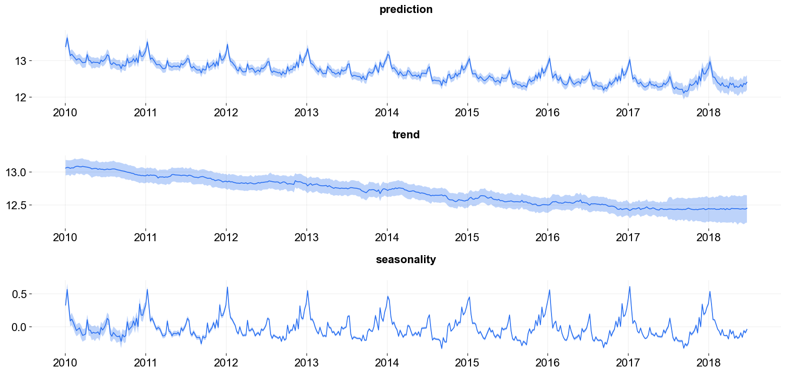
Also, users can request prediction with credible intervals of each component.
[11]:
predicted_df = ets.predict(df=df, decompose=True)
plot_predicted_components(predicted_df, date_col=date_col,
                          plot_components=['prediction', 'trend', 'seasonality'])
[11]:
array([<Axes: title={'center': 'prediction'}>,
       <Axes: title={'center': 'trend'}>,
       <Axes: title={'center': 'seasonality'}>], dtype=object)
Just like the MAPForecaster, one can also access the posterior samples by calling the function .get_posterior_samples().
[12]:
posterior_samples = ets.get_posterior_samples()
posterior_samples.keys()
[12]:
dict_keys(['l', 'lev_sm', 'obs_sigma', 's', 'sea_sm', 'loglk'])
As mentioned, in MCMC (Full Bayesian) models, the first dimension reflects the sample size.
[13]:
lev = posterior_samples['l']
lev.shape
[13]:
(400, 391)
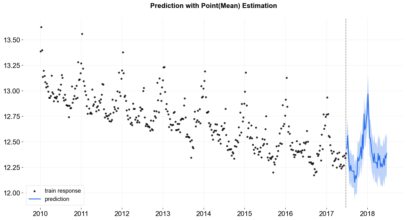
MCMC - Point Estimation
Users can also choose to derive point estimates via MCMC by specifying point_method as mean or median via the call of .fit. In that case, posteriors samples are first aggregated by mean or median and store as a point estimate for final prediction. Just like other point estimate, users can specify n_bootstrap_draws to report uncertainties.
[14]:
%%time
ets = ETS(
    response_col=response_col,
    date_col=date_col,
    estimator='stan-mcmc',
    seasonality=52,
    seed=8888,
    n_bootstrap_draws=1e4,
    stan_mcmc_args={'show_progress': False},
)

# specify point_method e.g. 'mean', 'median'
ets.fit(df=train_df, point_method='mean')
predicted_df = ets.predict(df=test_df)
2024-03-19 23:40:33 - orbit - INFO - Sampling (CmdStanPy) with chains: 4, cores: 8, temperature: 1.000, warmups (per chain): 225 and samples(per chain): 25.
CPU times: user 346 ms, sys: 245 ms, total: 591 ms
Wall time: 959 ms
[15]:
_ = plot_predicted_data(train_df, predicted_df, date_col, response_col,
                        title='Prediction with Point(Mean) Estimation')
One can always access the the point estimated posteriors by .get_point_posteriors() (including the cases fitting the parameters through MCMC).
[16]:
ets.get_point_posteriors()['mean'].keys()
[16]:
dict_keys(['l', 'lev_sm', 'obs_sigma', 's', 'sea_sm'])
[17]:
ets.get_point_posteriors()['median'].keys()
[17]:
dict_keys(['l', 'lev_sm', 'obs_sigma', 's', 'sea_sm'])